PLC PID Tuning Complete Guide: Kp, Ki, Kd for Real Industrial Loops

PID tuning is the controlled process of selecting proportional, integral and derivative behavior to meet explicit response and robustness objectives for a known loop. It starts after the measurement, actuator direction, scaling, execution interval, limits, modes and process constraints have been proven. Changing gains before those checks can hide a valve, sensor, timing or capacity fault without fixing it.

This guide explains the three terms, controller forms and units, pre-tuning proof, manual and model-based methods, a complete first-order-plus-dead-time calculation, saturation and anti-windup, manual/automatic transfer, acceptance tests and an evidence-led troubleshooting workflow. The arithmetic is vendor-neutral. Translate it only through the manual for the exact Siemens, Rockwell, CODESYS, Beckhoff, Schneider or other controller instruction; parameter names and units are not interchangeable.

Table of Contents

1. What PID Actually Does
2. The Three Terms in Plain English
3. PID in PLC Function Blocks
4. Method 1: Trial and Error (the honest one)
5. Method 2: Ziegler-Nichols
6. Method 3: Cohen-Coon
7. Anti-Windup: the Thing Everyone Forgets
8. Common Tuning Anti-Patterns
9. Process-Specific Guidelines
10. From Simulation to Real Hardware
11. Acceptance Tests
12. Frequently Asked Questions
13. Primary Sources

What PID Actually Does

A PID controller takes the error — the difference between the setpoint (what you want) and the process variable (what you're measuring) — and uses it to compute the manipulated variable (what the PLC tells the valve, the drive, or the heater to do).

In plain arithmetic:

output = Kp * error + Ki * ∫error·dt + Kd * d(error)/dt

That's it. Three terms summed together. Kp scales the current error, Ki integrates the history of the error, Kd looks at how quickly the error is changing. Everything else — tuning methods, anti-windup, cascade loops — is elaborations on those three terms.

The Three Terms in Plain English

Proportional (Kp) answers "how big is the error right now?" If the temperature is 10 °C below setpoint and Kp is 2, the proportional contribution is 20 units of heater output. Double Kp, double the response. Kp alone will get you close to setpoint quickly but leaves a persistent offset (steady-state error).

Integral (Ki) answers "how long have we been off?" If you're 1 °C below setpoint for 60 seconds, the integral accumulates 60 °C-seconds of error and ramps the output up until the offset vanishes. Integral is what eliminates steady-state error; too much integral causes overshoot and oscillation.

Derivative (Kd) answers "how fast is the selected differentiated signal changing?" In a suitable controller form it can add damping, but it is sensitive to measurement noise, sample time and filtering. Derivative on error can also create a setpoint kick; many industrial implementations allow derivative on PV. Add it only when the process model and response objective justify it, and verify the exact block's filter and units.

A PI controller is a defensible initial candidate for many self-regulating loops because it removes steady-state offset without derivative noise sensitivity. That is not a universal rule: integrating, inverse-response, long-dead-time, interacting or constraint-dominated processes may need a different tuning objective or control structure.

PID in PLC Function Blocks

Many PLC ecosystems provide one or more PID instructions or libraries. Their equations, languages, units, timing modes, tracking inputs, limit integration and autotune support differ materially. Record the exact controller, firmware, engineering release, instruction/library revision and controller form before translating any number.

Siemens TIA Portal — PID_Compact and related technology objects: use the current S7-1200/S7-1500 PID function manual for the exact CPU, instruction/version, operating mode, configured cycle and tuning procedure. Siemens documents gain and time parameters as well as pretuning/fine-tuning behavior, but the admissible process state and result still need an approved field procedure.

Rockwell Studio 5000 — PID, PIDE and PPID: choose the instruction supported by the controller, programming language and project architecture. Rockwell documents independent/dependent forms, update time, derivative selection, limits and manual/automatic behavior. Do not move Kp, Ki, Kd, reset-time or rate-time values between forms without the documented conversion.

CODESYS, Beckhoff, Schneider and other IEC-language environments: IEC 61131-3 standardizes programming languages, not one universal PID function block. Select the documented library and exact version. For example, CODESYS documents PID_FIXCYCLE, Beckhoff documents controllers including FB_BA_PIDCtrl, and Schneider publishes multiple PID library interfaces.

The transferable work is to prove signals and direction, establish deterministic timing, declare limits and modes, identify the process at the intended operating point, select an objective, translate the resulting parameters into the chosen block's form, and validate the entire loop. The PLC PID program guide owns the surrounding reusable implementation; this page owns gain selection and response evidence.

Method 1: Trial and Error (the honest one)

Manual iteration can be appropriate when a controlled model-identification test is permitted and the process response can be observed safely. It is not permission to push a production loop to instability.

Use an approved sequence whose increments and abort conditions come from the process hazard review, not a generic percentage:

1. Freeze the baseline. Export the as-found tuning, controller form, limits, filters, sample interval, mode behavior and synchronized trend.
2. Prove the loop in manual. Verify PV at multiple references, output direction, actual actuator feedback, response sign, operating range and constraint indications.
3. Choose one objective. Define permitted overshoot, rise/settling band, disturbance recovery, actuator travel and saturation recovery. “Looks better” is not a criterion.
4. Run one permitted stimulus. Prefer a manual-output step for process identification when operations authorizes it. A setpoint step also tests controller behavior and is not the same experiment.
5. Change one parameter or one model assumption. Use the exact block's form and units. Do not adjust gain, scaling and filters together.
6. Wait for adequate evidence. Slow thermal, level and composition processes may require long observation windows; stop by the declared PV, output, rate, alarm or equipment conditions.
7. Compare with the baseline. Evaluate the same operating point and disturbance class, then accept, refine or roll back.
8. Retest constraints and modes. A nominal response is incomplete without saturation, manual/automatic, equipment-unavailable, restart and bad/stale-PV cases.

Download the PID loop pre-tuning record, step-response calculation worksheet, and PID acceptance matrix. They keep assumptions, units and changes visible.

Method 2: Ziegler-Nichols

Ziegler–Nichols is a historic starting-rule family, not a universal commissioning procedure. The closed-loop ultimate-gain test deliberately approaches sustained oscillation and may be prohibited by process, product, environmental, equipment or safety constraints. Use it only with written authorization and explicit abort limits.

Ultimate gain method:

1. Set Ki and Kd to zero.
2. Increase Kp until the process oscillates with sustained, non-decaying oscillations at the setpoint. Call this gain Ku (ultimate gain).
3. Measure the period of oscillation. Call it Pu.
4. Apply the Ziegler-Nichols gains:

Controller	Kp	Ki	Kd
P only	0.5 × Ku	—	—
PI	0.45 × Ku	1.2 × Kp / Pu	—
PID	0.6 × Ku	2 × Kp / Pu	Kp × Pu / 8

The classic rules target a relatively aggressive quarter-amplitude-decay response. Actual overshoot and robustness depend on the plant, delays, nonlinearities, controller form and discretization. A mathematically valid result can still be unacceptable for quality or equipment constraints.

Treat the result as one candidate to validate against the declared objective. If the required experiment is not permitted, use an approved open-loop response, a trustworthy model or the documented vendor tuning workflow instead.

Method 3: Cohen-Coon

Cohen–Coon is another historic reaction-curve family for a self-regulating process approximated by a first-order-plus-dead-time model. Published tables use different dependent/independent and gain/time conventions. Do not paste a coefficient until its controller form and time units are reconciled with the PLC block.

1. Put the loop in manual mode.
2. Step the output by ~10 % and record the response.
3. From the response curve, measure:
   • Dead time (L) — time between step and first process variable movement.
   • Time constant (T) — time from first movement to 63 % of the final value.
   • Process gain (K) — (final PV change) / (output step).
4. Apply Cohen-Coon gains:

Controller	Kp	Ki	Kd
PI	(T / (K·L)) × (0.9 + L/(12T))	Kp × (L × (30 + 3L/T)) / (9 + 20L/T)	—
PID	(T / (K·L)) × (4/3 + L/(4T))	Kp × (L × (32 + 6L/T)) / (13 + 8L/T)	Kp × (4L / (11 + 2L/T))

Worked first-order-plus-dead-time identification

Assume an authorized manual-output step changes the applied output from 35% to 40%, so Δu = 5 percentage points. After settling, a temperature PV changes from 52.0 °C to 58.0 °C, so Δy = 6.0 °C. The observed delay before response is L = 12 s, and the PV reaches 63.2% of its final change 48 seconds after the response begins, so T = 48 s.

• process gain K = Δy / Δu = 6.0 / 5 = 1.2 °C per output percentage point;
• dead time L = 12 s;
• time constant T = 48 s; and
• normalized dead time L/T = 0.25.

This describes one operating point and direction. Repeat or validate the model if hysteresis, heating/cooling asymmetry, load, valve position or equipment lineup changes the response.

For a conservative IMC/lambda-style PI illustration, choose λ = 60 s and use the stated form Kc = T / [K(λ + L)], Ti = T. Then:

Kc = 48 / [1.2 × (60 + 12)] = 0.556 output-% per °C

Ti = 48 s

These are calculation outputs, not field-approved gains. Translate them into the exact PLC form: a block that accepts integral time receives Ti; a parallel form may require an integral gain derived with its documented equation and units. Record the model, formula source, parameter conversion and result in the worksheet before testing.

Anti-Windup: the Thing Everyone Forgets

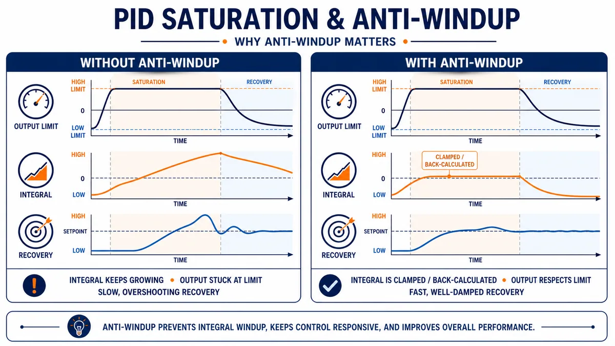
Integral windup occurs when integral action continues to store correction while the demanded process change cannot be applied. Here's one common sequence:

1. The process is stuck — maybe a valve is fully open but the flow won't reach setpoint because upstream pressure is low.
2. The integral term keeps accumulating error because the error won't go away.
3. The internal integrator grows to enormous values — far beyond what the actuator can physically deliver.
4. Conditions change, the process starts moving, the output should come down — but the stored integral keeps the request saturated during recovery.
5. The PV can overshoot or remain slow to recover while the internal state unwinds.

Fixes:

1. Clamp or condition integration. Depending on the documented implementation, integration is stopped or permitted only when it helps move the controller out of saturation. Verify how equality, direction, manual mode and internal/external limits are handled.

2. Back-calculation. The difference between requested and limited/applied output is fed back to correct controller state. The tracking gain/time is part of the design; an arbitrary value can create another transient.

3. External tracking. When a downstream selector, rate limiter, interlock or actuator constrains the demand, track the value actually applied if the block supports that architecture. Internal limits alone cannot see every downstream constraint.

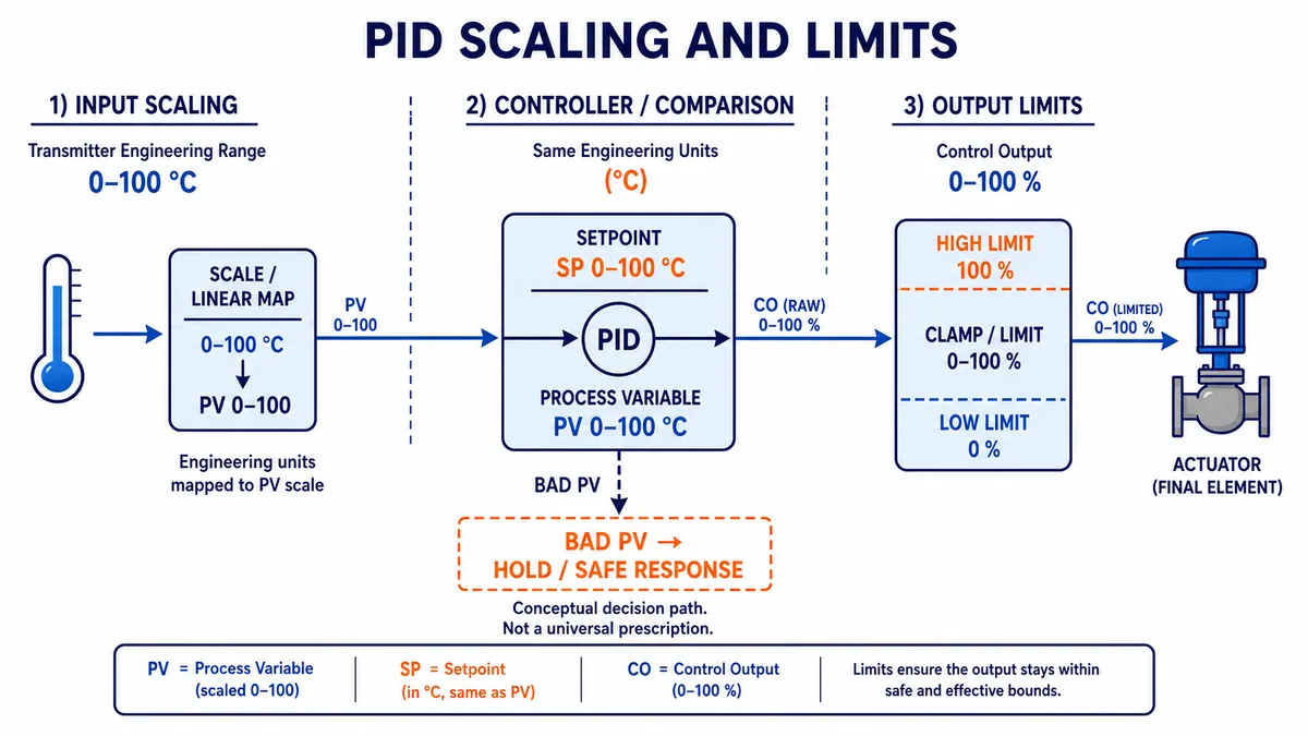
Set internal output limits consistently with the approved actuation envelope and expose requested, limited and applied outputs separately. A nominal 0–100% signal still may not equal actual valve position, VFD speed or heater duty. Anti-windup cannot compensate for wrong scaling, missing feedback, an unavailable actuator or an unreported downstream clamp.

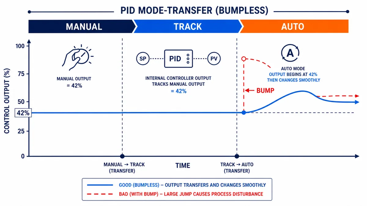
Bumpless manual-to-automatic transfer

A good nominal tuning can still create a dangerous bump if controller state does not match the applied manual demand. Before automatic ownership, prove the vendor-supported tracking path, effective output, setpoint behavior, controller action, active selectors and limit status. Test automatic-to-manual and manual-to-automatic transitions at more than one output, including a constrained condition. Do not achieve a cosmetically smooth transfer by hiding a stale or invalid PV.

Common Tuning Anti-Patterns

Seen too many times to count:

1. Copying tuning gains between loops. "This loop tunes at Kp=2.5, let me try that on the next one." Gains are dimensional — they depend on engineering-unit scaling, actuator range, and process dynamics. Never copy; always re-tune.
2. Turning off integral to "stabilise" a loop. A persistent oscillation is not fixed by removing integral. It means Kp is too high or the process has changed. Removing integral just gives you steady-state error plus the oscillation.
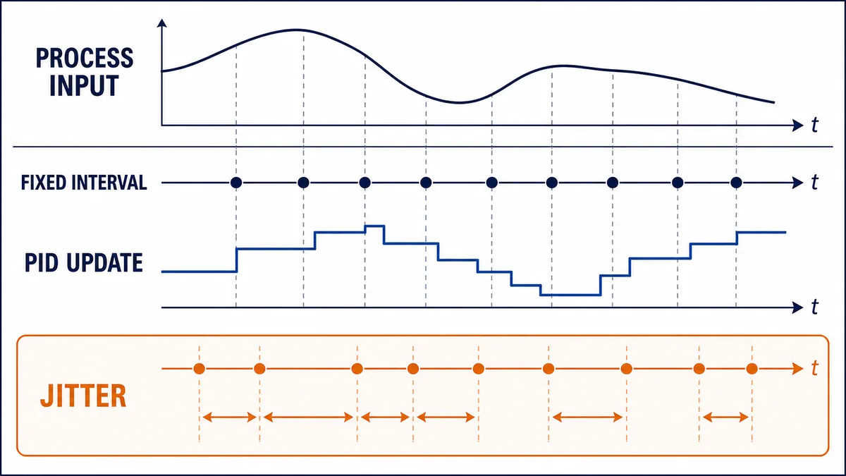
3. Adding derivative without a noise and timing review. Derivative can amplify measurement noise and sample jitter. Inspect the exact derivative input and filter before enabling it.
4. Leaving unexplained manual operation unresolved. A loop that remains manual may indicate a process, equipment, tuning, mode or trust problem. Record the reason and correct the underlying issue through change control.
5. Tuning at the wrong operating point. A valve with a linear characteristic at 50 % open has a non-linear characteristic at 90 % open. Tune at your normal operating range, not on a bench.
6. Tuning interacting or cascade loops as isolated SISO loops. Tune and validate the inner/secondary loop first, then select an outer-loop response that respects measured inner-loop dynamics and process interaction. Do not rely on a universal speed ratio.
7. Letting the PID drive outside physical limits. A PID output of 110 % means nothing to a valve that opens to 100. Clamp at the function block; don't rely on downstream logic.
8. Forgetting to disable PID during startup. Many processes need a specific startup sequence (pre-heat, pre-fill, flush) before PID control takes over. Starting PID from zero setpoint on a cold process often produces a wild first response. Use bumpless transfer from manual to auto.

Process-Specific Guidelines

Controller gains are dimensional and depend on scaling, controller form, execution interval and process dynamics, so a cross-industry table of “typical gains” is unsafe. Use a process-class table to decide what must be identified instead:

Process class	Evidence to identify	Tuning concern	Additional design question
flow or pressure	sensor/filter time, valve/VFD response, process gain and delay	fast timing, noise, stiction and interaction	is the final element sized and mechanically healthy?
temperature	heating/cooling asymmetry, transport delay, thermal time constant and capacity	long tests, output saturation and overshoot constraints	are there separate heat/cool outputs or gain schedules?
level	integrating/self-regulating behavior, inflow/outflow disturbances and geometry	objective may be surge absorption rather than tight SP tracking	is the vessel nonlinear or constraint-dominated?
composition or pH	analyzer delay, mixing, nonlinear gain and reagent authority	large operating-point changes can invalidate one tuning	is a nonlinear, split-range or model-based structure required?
cascade	inner-loop closed-loop response and cross-coupling	outer loop must respect actual inner dynamics	are modes, tracking and initialization coordinated?
override/selective	selector direction, active constraint and downstream applied output	windup and transfer between controllers	which controller tracks the selected output?

From Simulation to Real Hardware

A bounded simulator can make gain, delay, saturation, noise and disturbance effects visible without controlling installed equipment. Its result is valid for its disclosed model and numerical implementation—not automatically for the plant. Compare these layers explicitly:

Surface	Simulator can demonstrate	Hardware/plant evidence still required
controller arithmetic	declared parallel/ideal form, sample interval, limits and noise model	exact PLC instruction, task timing, precision, modes and firmware behavior
process	disclosed transfer function or numerical model	operating-point gain, delay, nonlinearities, interactions and unmeasured disturbances
measurement	injected noise, delay, bias and failure cases	transmitter calibration, wiring, filtering, quality and actual update age
actuator	commanded limit, rate and simple lag/stiction models	final-element feedback, deadband, stroke/ramp, availability and equipment constraints
safety	no physical consequence inside the teaching model	separate hazard controls, permits, interlocks and independently engineered safety functions

Use the simulator to form and test hypotheses: higher gain, slower integral, a changed sample interval, a stuck actuator, a bad sensor or a downstream clamp. Then create a separate authorized plant test with smaller allowed stimuli and explicit stop conditions. A model that matches one step at one operating point can diverge elsewhere.

Acceptance tests for a PLC PID loop

One attractive setpoint trend is not acceptance. Define numerical limits appropriate to the process, then execute the relevant cases while collecting aligned SP, PV, quality, requested/actual mode, raw/limited/applied output, constraints, equipment state and timestamps.

Test	Controlled condition	Passing evidence
1. configuration identity	exact CPU, firmware, engineering version, instruction/library and project revision	identity record agrees with approved source and online target
2. execution timing	normal and representative controller/network load	measured interval and jitter remain within the instruction/design requirement
3. PV scaling	low, middle and high independent references	engineering value, quality and raw channel agree within declared tolerance
4. output direction	small authorized manual output change	final element and PV move in the expected direction with no hidden inversion
5. output scaling	multiple manual commands	requested, limited and actual feedback reconcile with physical position/speed/duty
6. setpoint response	approved SP change at named operating point	overshoot, rise, settling band and output travel meet declared criteria
7. disturbance response	repeatable approved load disturbance	recovery and accumulated error meet the chosen objective
8. upper saturation	controlled upper constraint	limit visible; controller state does not cause unacceptable release recovery
9. lower saturation	controlled lower constraint	symmetric or documented asymmetric behavior passes
10. downstream constraint	selector/rate/interlock constrains applied demand	tracking/anti-windup uses the intended effective value and status is visible
11. manual to auto	transitions at multiple outputs	applied output stays inside permitted bump and mode ownership is unambiguous
12. auto to manual	operator or sequence transfers control	manual station inherits the intended applied demand without hidden jump
13. bad/stale PV	simulator or authorized signal-quality fault	approved hold, track, fallback or stop state occurs with correct alarm/evidence
14. actuator unavailable	equipment permissive removed under safe test	controller does not wind up invisibly or command unavailable equipment
15. restart/download	approved restart and restoration cases	modes, tuning, retained state, outputs and alarms match restart specification
16. regression	accepted cases rerun after final change	as-left tuning and project revision reproduce all required results

Diagnose before retuning

Symptom	First synchronized comparison	Candidate boundary	Avoid changing first
PV moves away from SP	small manual output step versus PV direction	action, scaling, wiring or process sign	gain magnitude
PV does not move	requested/limited/applied output and actual equipment feedback	availability, final element, process capacity or sensor	integral gain
output pinned high/low	error, constraint status, equipment feedback and disturbance	insufficient authority, wrong direction, clamp or load	all three gains together
repeating oscillation	oscillation period versus task, sensor, actuator and process delays	tuning, stiction, interaction, timing or dead time	filters and gains simultaneously
noisy/chattering output	raw/filtered PV, derivative term, task jitter and final-element deadband	signal/noise, derivative/filter, resolution or mechanics	setpoint
bump entering auto	applied manual output versus tracked/internal output and SP	mode tracking, selector or stale state	process gain model
slow recovery after limit	raw/limited/applied demand and integral/limit status	windup, unreported constraint or insufficient capacity	proportional gain only
response changed after software work	actual cycle, PV age, block form and restored parameters	timing/configuration regression	plant equipment

PID references and platform-specific implementations

If you first need the terms and loop anatomy, use the PID control reference. For architectures beyond one loop, compare advanced process-control strategies. For implementation after the controller family is known, follow the dedicated Delta PID program example, FX5U PID implementation guide or RSLogix 5000 PID implementation guide rather than translating gain values or instruction behavior by name alone.

Frequently asked questions

How do I tune a PID loop in a PLC?

First prove PV scaling and quality, output direction and feedback, deterministic execution timing, controller form, limits, modes, interlocks and available equipment. Define response criteria, then run an approved manual-output step or another documented identification method. Estimate the process, calculate a conservative candidate, translate it into the exact PLC block's units, and validate setpoint, disturbance, saturation, transfer, restart and fault cases. Save the as-found and as-left evidence.

What do Kp, Ki and Kd mean?

Kp scales current error, Ki or integral time controls accumulated-error action, and Kd or derivative time controls response to a rate of change. Those names do not guarantee identical equations. Parallel, ideal/dependent, series and two-degree-of-freedom forms use different parameter relationships; PLCs may express integral/derivative as gains or times. State the equation, PV/output units and time base before comparing numbers.

Should I tune Kp before Ki and Kd?

A P-then-I workflow can help isolate behavior in a permitted manual tuning exercise, and starting without derivative reduces variables. It is not a license to increase proportional gain until an installed process oscillates. When a trustworthy step-response model exists, a model-based PI candidate may avoid that experiment. In either case, change one justified parameter, keep abort criteria, and compare against the same objective.

What is the difference between Ki and Ti?

Ki commonly denotes integral gain, while Ti commonly denotes integral or reset time. In one ideal/dependent continuous form, integral action contains Kc/Ti; in a parallel form the independent coefficient can be Ki. Exact conversions depend on the manufacturer's equation and time units. A value of 1 can mean per second, repeats per minute or a time; never transfer it by label alone.

What is Ziegler-Nichols PID tuning?

It is a classic family of empirical rules. The closed-loop method identifies ultimate gain and oscillation period; reaction-curve rules use a process response. The resulting candidate is often aggressive and the ultimate-gain experiment may be unacceptable on a production process. Confirm the specific published rule, controller form and units, obtain authorization, and validate against process-specific overshoot, robustness, actuator and quality constraints.

What is Cohen-Coon tuning?

Cohen–Coon uses an open-loop reaction curve approximated by process gain, dead time and time constant. It is one historic option for a self-regulating first-order-plus-dead-time approximation. Formula tables differ in controller form and whether they report integral/derivative gains or times. Record the source and translation; do not assume a coefficient copied from one table matches a PLC block.

What is lambda or IMC PID tuning?

Lambda/IMC-style tuning chooses a desired closed-loop speed or robustness parameter, often called λ, from a process model. A larger chosen lambda generally requests a slower, more robust response for the stated model. There are different formulas for self-regulating, integrating, PI and PID cases. The worked example on this page declares its formula and units; it is not a universal recipe.

What is integral windup?

Integral windup is excessive stored integral action while the requested correction cannot be applied, such as during output saturation, equipment unavailability or a downstream selector. Recovery can remain delayed after the constraint clears. Use the exact block's clamping, back-calculation or tracking facility, expose raw/limited/applied demand, and test both saturation directions plus downstream constraints.

What is bumpless transfer in PID control?

It means the effective command stays within an approved change when ownership moves between manual and automatic control. Usually the controller's internal output/state must track the value actually applied, including downstream selectors and limits. Setpoint tracking is a related but separate choice. Test transfers at several outputs and constraints; do not infer bumpless behavior from a configuration label.

Should derivative act on error or process variable?

Derivative on error reacts to setpoint changes and can create a large output kick. Derivative on PV avoids differentiating the setpoint step but still responds to measurement noise and process movement. The right choice depends on reference-tracking versus disturbance objectives, controller form and filtering. Use the exact instruction option and validate with representative setpoint, disturbance, noise and task-timing cases.

How often should a PLC PID execute?

At a stable interval supported by the instruction and appropriate to the measured process dynamics. The configured time base must match actual execution, and sensor/network/output updates also affect end-to-end age. Faster execution is not automatically better; jitter, stale inputs or an actuator that updates much more slowly can invalidate assumptions. Measure the interval under representative controller load.

Can PID tuning fix a sticking valve or undersized heater?

No. Tuning cannot remove mechanical stiction, calibration error, wrong action, signal delay, insufficient capacity, a hidden clamp or equipment unavailability. It may move or mask the symptom. Compare requested, limited and applied output with actual final-element feedback and PV response, correct the failed boundary, then decide whether retuning is still required.

Can I copy PID gains from another loop?

Not safely. Gains depend on controller form, PV and output scaling, time units, execution interval, process gain, delay, operating point, actuator and response objective. Even nominally identical assets can differ through valves, sensors, loads and configuration. You can use the other loop as a hypothesis only after comparing a complete manifest and identifying the target process.

Can a browser PID simulator validate my plant tuning?

No. It can validate the disclosed teaching model and help you recognize gain, delay, noise, saturation and disturbance patterns. It cannot reproduce your PLC instruction, firmware, task timing, signal chain, final element, interacting plant or safety functions without a validated model and integration. Use it to prepare cases and improve diagnosis, then follow the site's authorized commissioning procedure.

Key takeaways

• Tuning begins after signals, direction, timing, limits, modes and equipment are proven.
• State the controller equation, parameter form, units and execution interval before comparing gains.
• Use a permitted stimulus and explicit objective; never pursue oscillation without authorization and abort limits.
• Preserve requested, limited and applied output so saturation and downstream constraints remain visible.
• Test transfer, restart and faults as well as nominal setpoint response.
• Keep as-found/as-left records, synchronized trends and a rollback condition.

Primary sources and review scope

This article was reviewed on 31 August 2026 against current manufacturer, standards-owner and control-tool documentation. Product behavior changes by controller, firmware, engineering release and library version; retrieve the exact applicable manual before implementation.

1. PID theory and coefficients — National Instruments
2. PID Control Toolkit User Manual — National Instruments
3. S7-1200/S7-1500 PID Control Function Manual, November 2025 — Siemens
4. S7-1200 System Manual V4.7 — Siemens
5. Logix PID instruction — Rockwell Automation
6. Using PID instructions and gain forms — Rockwell Automation
7. Anti-reset windup and bumpless transfer — Rockwell Automation
8. PID configuration, update time and derivative selection — Rockwell Automation
9. PID_FIXCYCLE function block — CODESYS
10. FB_BA_PIDCtrl — Beckhoff Automation
11. TwinCAT 3 Temperature Controller TF4110 — Beckhoff Automation
12. FB_PID — Schneider Electric
13. ControlLoopLibrary — Schneider Electric
14. PID Controller block forms and options — MathWorks
15. Anti-windup clamping, back-calculation and tracking — MathWorks
16. PID controller tuning and robustness — MathWorks
17. IEC 61131-3:2025 publication record — IEC
18. Control of hazardous energy, 29 CFR 1910.147 — OSHA

The figures are original conceptual/editorial illustrations, not vendor screens, controller code, P&IDs, electrical drawings, safety architectures or field approvals. This article does not authorize connecting, forcing, bypassing, tuning, starting or testing installed equipment. Qualified personnel must follow the process hazard review, hazardous-energy and electrical safe-work requirements, approved operating envelope, exact manufacturer instructions and controlled change/commissioning procedure.

Related reading

• Temperature control PLC programming guide
• Pump control PLC programming guide
• VFD programming PLC control guide
• PLC programming best practices
• PLC PID program implementation
• Worked PID control-system calculation
• PID project briefs and acceptance evidence