PID Projects for PLCs: 8 Labs with Test Plans

Direct answer

A good PLC PID project is a small closed-loop system with one controlled variable, one manipulated variable, a documented disturbance, a repeatable process model, explicit operating modes and measurable pass criteria. The best first project is a virtual temperature chamber: temperature is the process variable (PV), heater demand is the control output (CV or MV), heat loss is the disturbance, and the learner can see delay, overshoot, settling, saturation and recovery without energizing a real heater.

Do not judge the project by whether the trend eventually reaches setpoint. A complete project proves signal scaling and quality, output direction, fixed controller timing, manual-to-automatic transfer, output limits, setpoint tracking, disturbance rejection, sensor-fault behavior, actuator constraints and repeatable recovery. Retain the requirements, configuration, scenario definition, synchronized trends, calculations and pass/fail decision so another person can reproduce the result.

This page uses PID projects in the control-engineering sense. The singular search phrase “PID project” is commonly used for a Project Initiation Document in project management; that is not the topic here. For the reusable controller-module implementation, use the PLC PID program guide. For detailed gain-selection and tuning-method theory, use the PLC PID tuning guide.

PID project quick-selection table

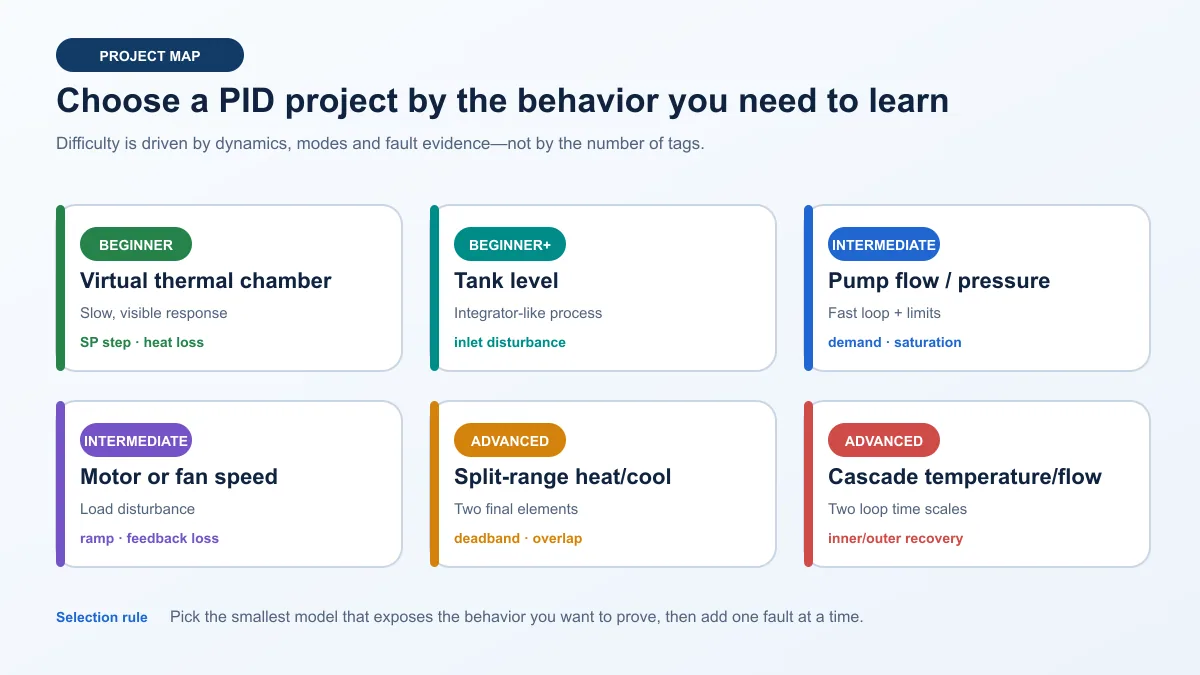
Choose a project for the behavior you need to learn. Do not begin with cascade or split-range control because it sounds impressive; begin with a loop whose cause and effect you can predict.

Project	Controlled variable	Manipulated variable	Designed disturbance	Main lesson	Starting level
virtual thermal chamber	temperature	heater demand	door opening or ambient heat loss	delay, setpoint response and output limiting	beginner
virtual tank level	liquid level	outlet-valve demand	inlet-flow step	accumulation, direction and saturation recovery	beginner+
pump flow	flow rate	pump-speed demand	downstream restriction or demand change	fast response, noise and minimum speed	intermediate
pressure control	header pressure	pump, fan or valve demand	consumer demand step	capacity limit and disturbance rejection	intermediate
motor or fan speed	rotational speed	drive torque/speed demand	load-torque step	fast loop, feedback loss and command ramps	intermediate
split-range temperature	temperature	heating and cooling demands	heat-load step	two final elements, overlap and deadband	advanced
cascade temperature/flow	temperature outer loop	flow setpoint to inner loop	supply or heat-transfer change	time-scale separation and mode coordination	advanced
diagnostic challenge	selected PV	selected actuator demand	noise, bias, stiction, delay or capacity loss	distinguish process, sensor, controller and actuator faults	intermediate–advanced

The row is a project brief, not a hardware instruction. A real pump, fan, motor, pressure vessel, heater or energized panel introduces electrical, mechanical, thermal, hydraulic and stored-energy hazards that a web page cannot assess. Build the first version in a deterministic simulator. Move to physical equipment only under an approved design, qualified supervision and the applicable safe-work process.

What makes a PID controller project complete?

A project needs a question, not just a process

“Control temperature” is a topic. “Hold a virtual chamber at 28 °C after a 20% increase in modeled heat loss, with no more than 2 °C overshoot, no unexplained output saturation and recovery inside the agreed time band” is a testable project question. The second statement identifies the controlled variable, disturbance, response constraint and evidence needed for a decision.

State which performance matters. Setpoint tracking asks how the loop follows a requested target. Disturbance rejection asks how it restores the process after an external load changes. Those objectives can require different compromises; a controller that follows setpoints aggressively can overshoot, amplify noise or reject load changes poorly. Test them separately before combining them.

Define six project artifacts before programming

Artifact	Minimum content	Why it matters
one-page requirement	objective, normal range, limits, modes, disturbances and pass criteria	prevents retrospective success criteria
I/O and state contract	PV, SP, requested/limited/applied output, quality, mode and reason tags	separates values that look similar but mean different things
process-model note	equations or behavior, units, sample interval, delay, saturation and assumptions	makes simulation results interpretable
test matrix	baseline, setpoint, disturbance, limit, quality, mode and recovery cases	proves more than the happy path
evidence bundle	configuration revision, timestamped trends, calculations and observations	makes the result repeatable and reviewable
transfer boundary	what simulation proves and what requires approved hardware testing	prevents a model result from becoming a safety or commissioning claim

Separate controller calculation from project orchestration

The PID function computes a correction. The project also needs signal validation, mode arbitration, manual demand, tracking, output selection, constraints, equipment availability, alarms, trend points, fault injection and reset/recovery rules. Hiding all of those responsibilities inside a single opaque “PID working” Boolean makes the lab hard to diagnose and teaches the wrong engineering habit.

Expose at least these values: setpoint, raw PV, validated PV, PV quality and age, error, raw PID output, limited output, applied output, requested mode, effective mode, active constraint, actuator availability and first-out inhibit reason. If the selected platform exposes proportional, integral and derivative contributions, trend them during diagnosis, but do not assume every vendor defines those fields identically.

Use a requirement-to-evidence workflow

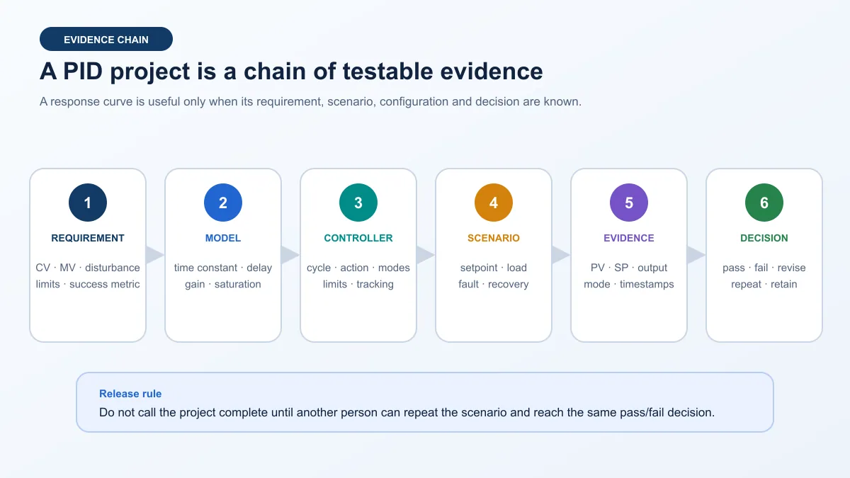
A response curve is useful only when its requirement, scenario, configuration and decision are known. Treat those four links as a release contract: if one is missing, preserve the run as exploratory evidence rather than a passed project test.

Step 1: write the control objective

Name the controlled variable (CV in process-engineering language, often PV in controller interfaces), manipulated variable (MV, frequently called controller output or CV by PLC vendors), setpoint, expected disturbances and normal operating region. Because vendors use “CV” differently, define every abbreviation in the project rather than arguing from a screenshot.

Include the direction of process gain: when the applied output increases, does the process variable eventually rise or fall? Do not derive that direction from “fail open,” “cooling,” or a direct/reverse label. Those words describe different aspects of the loop. Prove the modeled direction manually, then verify the exact vendor meaning before selecting controller action.

Step 2: define the model boundary

A learning model need not reproduce every physical effect. It must reproduce the effects the test claims to evaluate. A temperature project that evaluates overshoot and settling needs stored heat, heat input, heat loss and a repeatable sample interval. A level project needs accumulation: level changes with the difference between inlet and outlet flow. A flow project needs a faster response, meaningful limits and optionally measurement noise.

Record model units, initial conditions, process gain, time constant or response rate, dead time, nonlinearities, saturation, noise and disturbance inputs. If you change a model parameter during a comparison, label the run as a different plant. Otherwise an apparent tuning improvement may only be an easier model.

Step 3: select the supported controller form

Siemens, Rockwell Automation, Schneider Electric, AutomationDirect and IEC-library implementations differ in algorithm form, gain units, calling pattern, tracking, limits and available languages. Use the exact controller family, software release and current documentation. Do not translate a gain or integral time by label alone.

The project page remains vendor-neutral. Its contract is “validated PV and SP enter a documented controller at a known interval; raw output passes through known limits and mode logic to become applied demand.” The PID program implementation owner covers that wrapper in depth.

Step 4: define scenarios before tuning

A scenario is a controlled change with a baseline, start time, one intentional stimulus and a defined observation window. Useful stimuli include a setpoint step, ramped setpoint, load disturbance, output limit, measurement bias, sensor noise, data-quality loss, actuator deadband, actuator stiction, capacity loss and mode transfer. Change one boundary at a time when the goal is diagnosis.

Step 5: calculate metrics from the same window

Use the same baseline and observation rules across variants. At minimum calculate peak overshoot, settling time, final or steady-state error, time spent at an output limit and a simple integrated-error measure. Add actuator travel or output movement when wear matters. A pretty trend without a time base, units or acceptance band is weak evidence.

Step 6: retain the decision

Record whether the run passed, failed or was invalid. “Invalid” is necessary when the initial condition was wrong, the model changed unexpectedly, the trace was missing, two faults were injected, or a controller was not actually in the intended mode. Preserve failed and invalid runs; they show that the test system can detect problems rather than only produce success screenshots.

Project 1: virtual PID temperature-control chamber

Why temperature is the best first project

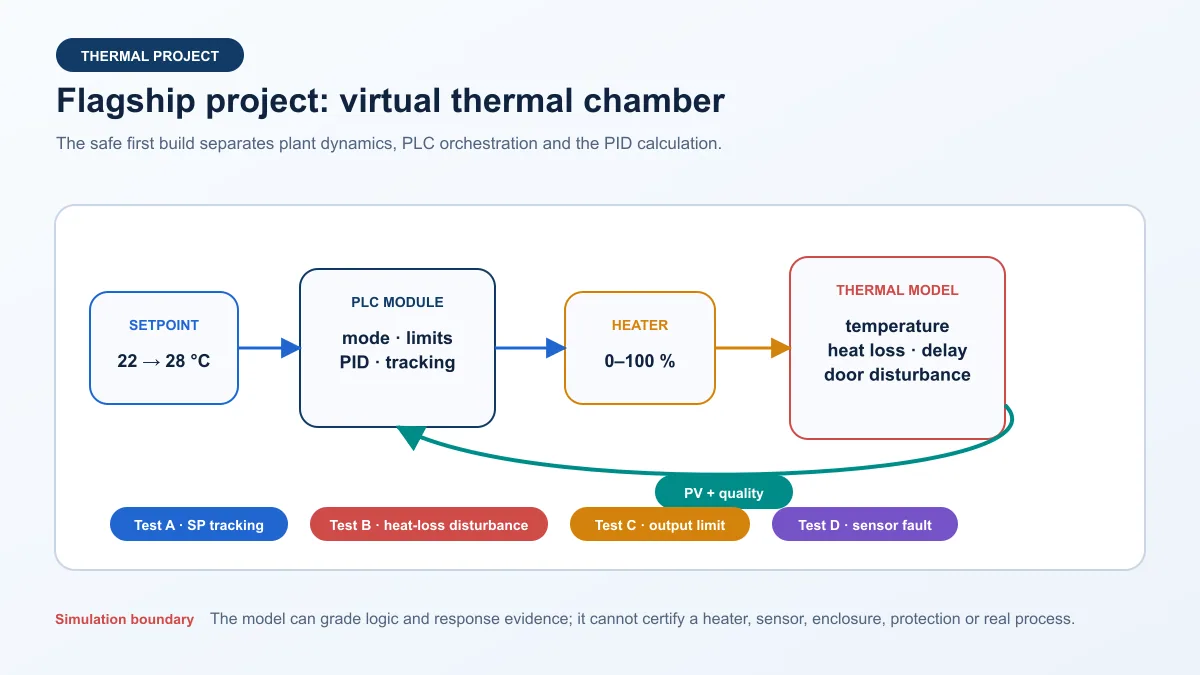
A first-order thermal model changes slowly enough to observe. It shows why increasing output does not produce an immediate PV jump, why aggressive integral action can accumulate during a limit, and why the loop continues moving after output changes. The learner can run the same model repeatedly without the electrical design, thermal protection, fire risk and stored heat of a physical heater.

The project’s controlled variable is chamber temperature in degrees Celsius. The manipulated variable is a bounded 0–100% modeled heater demand. The primary disturbance is modeled heat loss, which can change at a known time to represent an opened door, colder ambient condition or increased airflow. The model exposes temperature, heater demand, heat-loss setting and an optional sensor-quality state.

Use a transparent model

A simple discrete model can express the teaching behavior:

T_next = T_now + Δt × (heater_gain × applied_output − loss_gain × (T_now − ambient)) / thermal_capacity

Every quantity needs units or a declared normalized interpretation. Δt must match the model update interval. The model is editorial and educational; it is not a heat-transfer design or a promise that a real chamber has the same gain, delay, efficiency or safe limit.

Model item	Example learning value	Required note
initial chamber temperature	22 °C	same baseline for comparisons
ambient temperature	20 °C	disturbance reference, not measured room claim
setpoint	28 °C	bounded inside project range
model interval	100 ms	fixed and recorded
output	0–100%	normalized modeled demand
output limit test	45% maximum	deliberate constraint for anti-windup observation
door/heat-loss step	at 300 s	one controlled disturbance time
sensor fault	bad quality at 500 s	mode response defined before run

Build the surrounding state model

Use INITIALIZING, MANUAL, TRACK, AUTOMATIC and UNAVAILABLE as explicit effective states, or an equally clear platform-specific model. Start in manual or track. Let the operator or test harness set a bounded manual heater demand. When transferring to automatic, align controller state to applied output so the first automatic calculation does not create an unrelated bump.

Do not simply stop calling the controller when sensor quality goes bad. Depending on the function block, skipped calls can freeze state or violate timing assumptions. Use the documented manual, track, hold or degraded mechanism and keep the plant-level applied output behavior separate. There is no universal safe physical fallback, so the simulator must label its choice as a project rule rather than field advice.

Run four required tests

1. Setpoint tracking: begin from the same stable baseline, step from 22 °C to 28 °C, and measure rise, overshoot, settling, final error and output-limited time.
2. Heat-loss rejection: keep setpoint constant, increase modeled loss at a recorded time, and measure maximum deviation and recovery.
3. Output constraint: lower the maximum applied demand while the loop is below setpoint, then restore it and inspect integral recovery and raw-versus-applied output.
4. Sensor-quality loss: mark PV bad or stale, confirm the defined effective mode and output response, restore quality, and prove deliberate bumpless recovery.

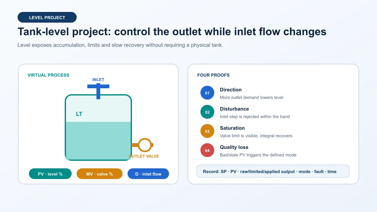
Project 2: virtual tank-level control

Make the process relationship explicit

Use level as PV, outlet-valve demand as the manipulated variable and inlet flow as the disturbance. With that arrangement, increasing outlet demand should eventually lower level. The controller action must reflect the proven process direction and the selected vendor’s definition.

A basic model updates vessel volume from the flow difference, then converts volume to level using the vessel cross-sectional area. Clamp the physical model at empty and full conditions while retaining an at_low_boundary or at_high_boundary state. Do not let the model silently calculate negative volume or an impossible level and then declare the controller unstable.

Test accumulation and saturation

Level is an integrating process: a sustained flow imbalance continues changing inventory. Begin with inlet and outlet balanced. Step inlet flow while setpoint remains constant. The controller should increase outlet demand and restore level without hiding that the valve reached a limit. Then constrain the outlet so inflow exceeds maximum outflow; a good project should show that no tuning value can overcome missing capacity.

Test	Stimulus	Evidence	Valid conclusion
action proof	small manual outlet step	level slope changes in predicted direction	action can be selected from evidence
inlet disturbance	known inlet-flow increase	PV deviation, output movement and recovery	disturbance rejection at this operating point
capacity loss	reduce maximum outlet flow	raw/limited/applied output and continuing level rise	equipment authority is insufficient
quality loss	stale or invalid level	effective mode, applied demand and reason	degraded behavior matches the project rule
restart	save state, reset controller/module	initial mode, PV, SP and output	restart is deterministic for the tested condition

Project 3: pump-flow PID project

Use a fast model and expose noise

Flow normally responds faster than temperature or level. Model a pump or valve command, a short process lag, a bounded flow range and a downstream-resistance disturbance. Add optional zero-mean measurement noise as a controlled input with a saved seed so comparisons are repeatable.

Start with PI behavior unless the project explicitly evaluates derivative filtering. This is not a universal plant prescription; it is a clean experimental design. Compare raw PV, filtered PV, controller output and actuator movement. If a filter reduces apparent noise but delays the feedback enough to harm the response, the trend should reveal the tradeoff.

Add minimum and maximum operating constraints

A modeled pump may have a minimum useful speed and a maximum capacity. Represent those as project constraints, not hidden clamps. Trend raw controller request, limited speed request and applied model input. When the flow setpoint is unreachable, the pass condition is not “PV reaches SP”; it is “the project identifies sustained saturation, retains the error and reports insufficient authority without an unsafe or fabricated remedy.”

Project 4: pressure or fan-speed disturbance rejection

Distinguish command following from load rejection

For a pressure model, keep setpoint constant and step consumer demand. For a fan or motor-speed model, keep speed setpoint constant and step load torque. These tests isolate disturbance rejection from setpoint tracking. Record maximum deviation, recovery time and output movement.

Do not compare two controllers using different load steps or initial conditions. Save the model state, controller state and configuration. If the simulator cannot restore state deterministically, run a documented warm-up period and use an objective baseline criterion such as PV inside a narrow band with output stable for a defined duration.

Test lost feedback and actuator availability

Inject a feedback-quality loss separately from a process disturbance. Then make the actuator unavailable while feedback remains valid. The two cases should produce different first-out reasons even if both stop automatic control. This distinction is valuable in a real troubleshooting workflow: a plausible PV does not prove the actuator is available, and an available actuator does not make a stale PV safe to control from.

Project 5: split-range heating and cooling

Give each final element a visible allocation

A split-range project converts one controller demand into two applied outputs, such as heating and cooling. Define the split point, overlap or gap, output characterization, limits and which applied output the controller tracks. The educational objective is not to recommend simultaneous heating and cooling; it is to expose how a selector and two nonlinear final elements change the loop.

Controller demand	Heating allocation	Cooling allocation	Project question
0–40%	decreasing toward zero	active according to defined map	does cooling respond and release predictably?
40–60%	gap, overlap or neutral band by design	gap, overlap or neutral band by design	is the transition observable and intentional?
60–100%	active according to defined map	decreasing toward zero	does heating enter without a demand bump?

The numbers are an example mapping, not a universal convention. Reverse the outputs if the project definition requires it. Test both directions through the split region, introduce modeled deadband, and show requested versus applied heating/cooling separately. A single “output percent” trend hides the main lesson.

Project 6: cascade temperature and flow

Make the inner loop demonstrably faster

The outer temperature controller writes the inner flow setpoint; the inner flow controller drives the final element. First commission and grade the inner loop by itself. Its response should be materially faster than the outer loop’s dynamics for the cascade structure to make sense. Do not quote a universal 3:1 or 5:1 rule as proof; measure the chosen models and define an acceptance margin.

Test mode coordination

Specify what happens when the inner loop goes manual or becomes unavailable. The outer loop should not continue integrating as though its requested flow setpoint is being applied. Trend outer raw output, inner SP, inner PV, inner applied output and both effective modes. Test return to cascade with tracking so neither controller creates a hidden bump.

Scenario	Inner loop	Outer loop	Evidence required
normal cascade	automatic, accepts remote SP	automatic	both loops settle and constraints are visible
inner manual	manual demand applied	track/hold behavior defined	outer state follows what can actually be applied
inner unavailable	no normal automatic control	degraded state defined	first-out cause and outputs are explicit
recovery	available and tracked	deliberate return to cascade	no unexplained SP or output step

Project 7: noisy measurement and filtering comparison

Use identical noise and model conditions

Create a saved noise sequence or deterministic seed. Run the same controller with no filter, a light filter and a deliberately excessive filter. Compare PV variance, output movement, setpoint response and disturbance recovery. This prevents “the filtered run looks smoother” from becoming the only conclusion.

Include a bias fault as a separate test. A low-pass filter can reduce high-frequency variation but cannot remove a steady sensor bias without changing the meaning of the measurement. The controller may hold the displayed PV at setpoint while the underlying true model variable is wrong. Trend both true model value and observed PV in the lab, label the former as simulation-only truth, and explain that real plants do not normally expose a perfect hidden value.

Project 8: saturation, stiction and recovery diagnostic challenge

Seed one fault without naming it to the learner

Create a known-good baseline, then inject one of four faults: an output clamp, actuator deadband, actuator stiction or process-capacity loss. Give the learner SP, PV, raw/limited/applied output, mode, quality and actuator feedback. Ask for a diagnosis, evidence citation and the next safe test—not a tuning change.

The challenge should distinguish a controller at 100% because the process needs more authority from an actuator that was commanded to 100% but applied only 55%. It should also distinguish repeated stick-slip movement from a controller oscillation. A grading rubric can award points for identifying the first divergence in the evidence chain, rejecting unsupported conclusions and proposing a single discriminating test.

Write the PID project specification

Define signals as contracts

Use names that preserve meaning across the project. PID_Output is ambiguous when a selector, ramp, clamp or unavailable actuator changes the value downstream. Prefer explicit roles such as PID_RawDemand, DemandAfterLimits, AppliedModelDemand and ActuatorFeedback. The exact tag syntax varies, but the semantic separation should survive translation.

Signal role	Example name	Units/state	Contract question
requested setpoint	Temp_SP_Request	°C	who may write it and within what range?
effective setpoint	Temp_SP_Effective	°C	what ramp, selector or limit has been applied?
raw measurement	Temp_PV_Raw	input representation	what source and update interval produced it?
validated measurement	Temp_PV	°C	what scaling and plausibility checks passed?
measurement quality	Temp_PV_Quality	good/bad/stale/simulated	which state transitions change control mode?
PID request	Heater_PID_Raw	%	what does the controller calculate before constraints?
limited demand	Heater_Demand_Limited	%	which active limit changed it?
applied demand	Heater_Demand_Applied	%	what value actually enters the plant model?
effective mode	Temp_Mode_Effective	enum	what state truly owns output now?
first-out reason	Temp_Inhibit_FirstOut	enum/code	why could normal automatic control not continue?

The I/O contract must also state update ownership. A simulation task should not write the same PV tag as a real input mapper. Use an explicit source selector and conspicuous simulated-state indication. On real OT systems, control access, test accounts, remote access, backups and recovery belong to the approved security architecture; a learner project is not authority to add a hidden simulation path to production code.

Define controller and model timing separately

Record at least three intervals: model update, measurement publication and controller execution. They may be identical in a small lab, but keeping them explicit makes jitter, stale data and rate mismatch testable. The selected controller instruction may measure elapsed time internally, require a configured cycle, or expect a particular periodic task. Follow its current documentation.

Timing check	Pass evidence	Common invalid result
controller cycle configured	configured value matches supported calling pattern	value copied from another platform
controller actually executes	measured interval and overrun evidence retained	“periodic” inferred from code position
model updates predictably	timestamp increments and missed updates visible	model tied to variable UI refresh
PV age is known	quality becomes stale at defined maximum age	unchanged value assumed valid forever
trend samples are adequate	time base captures relevant rise and limit events	sparse samples hide peak or chatter

Predeclare project assumptions

State that the plant is a model; its parameters are selected for learning; its sensor is ideal unless a fault is injected; output is normalized; protection behavior is outside the PID algorithm; and no model result certifies hardware. When a project includes a physical low-voltage trainer, add the exact hardware, enclosure, power source, protection, sensor, actuator, drawing revision and approved procedure. Do not allow “24 VDC” to become a synonym for “risk free”; motion, heat, stored energy, sharp mechanisms and incorrect wiring can still cause harm.

Measure PID project performance

Peak overshoot

For an upward setpoint step with a stable final target, calculate:

overshoot % = 100 × (peak PV − final target) / |final target − initial PV|

The denominator must represent the requested change, not simply the target value. If the target did not remain constant or the process did not settle, label overshoot as not applicable or invalid instead of forcing a number.

Settling time

Define a tolerance band before the run, such as ±2% of the commanded change or a project-specific engineering-unit band. Settling time is the elapsed time from the stimulus until PV enters and remains inside that band for the declared dwell. If the observation window ends before the dwell completes, report “not settled within window.”

Steady-state error

Average error over a stable final window rather than selecting the last sample. Record the window start, duration and sample count. A small displayed error while the controller output is saturated can be temporary and should not be interpreted as proven capacity.

Integrated error

Integrated absolute error (IAE) is easy to compare:

IAE ≈ Σ |SP[k] − PV[k]| × Δt

Integral squared error penalizes larger errors more strongly; integrated time-weighted absolute error penalizes errors that persist. Choose one before comparing configurations and keep units, interval and run length consistent.

Output movement and saturation

Record maximum and minimum applied output, total time at each limit, and a simple movement measure such as the sum of absolute changes. This adds an actuator-effort dimension. A tune that reduces IAE slightly while doubling command movement may be undesirable for a valve or drive, though a simulator cannot predict actual wear without a validated actuator model.

Metric	Requirement example	Evidence note
peak overshoot	≤ 10% of requested change	final target and initial PV identified
settling time	≤ 240 s inside ±0.3 °C for 30 s	sample interval and dwell recorded
steady-state error	absolute mean ≤ 0.1 °C in final 60 s	valid only if process is stable
IAE	lower than saved baseline under identical scenario	same units, duration and model
high-limit duration	≤ 45 s unless case deliberately tests saturation	raw and applied output both retained
output movement	no unexplained high-frequency chatter	calculation and filter state documented
mode integrity	no uncommanded transition	requested/effective mode and first-out retained

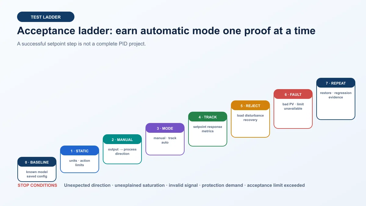
Use a staged acceptance ladder

Stage 0: baseline and reproducibility

Save the model version, controller program, parameters, initial state, simulator version and test-matrix revision. Run the unchanged baseline twice. If results differ materially, fix nondeterministic timing, unseeded noise or incomplete state reset before comparing tuning.

Stage 1: static configuration

Review signal units, ranges, action definition, cycle, controller form, limits, quality rules, mode transitions and reset behavior. Static review cannot prove the process response, but it can catch contradictions before they create misleading trends.

Stage 2: manual direction and authority

With normal automatic calculation not owning output, apply small bounded test demands in the model. Prove the correct modeled final element, response direction, useful output range and approximate delay. If the process does not move, do not tune.

Stage 3: mode and tracking

Test initializing to manual or track, manual-to-auto, auto-to-manual, unavailable entry, recovery and restart. Confirm the first automatic output aligns with the previously applied demand within the project tolerance. Track the value actually applied after downstream selection and limits.

Stage 4: setpoint response

Run the predeclared step or ramp. Calculate metrics from the saved trace. Do not change limits, model parameters or the stimulus midway. A human can stop an unsafe physical test, but that stopped run must be marked invalid or failed according to the predeclared rule—not edited into a clean demonstration.

Stage 5: disturbance rejection

Return to the same baseline, keep setpoint constant and apply the declared process disturbance. Measure deviation and recovery. This stage answers a different question from setpoint tracking and deserves its own acceptance criteria.

Stage 6: boundaries and faults

Exercise output limits, bad/stale PV, actuator unavailable, model capacity loss and one controlled sensor or actuator fault. Confirm that the expected evidence changes at the correct layer and recovery is deliberate.

Stage 7: repeat and review

Restore the baseline, rerun representative normal and fault cases, and ask another person to reproduce at least one decision. Package the requirements, test matrix, traces, calculations, failed runs, configuration and limitations.

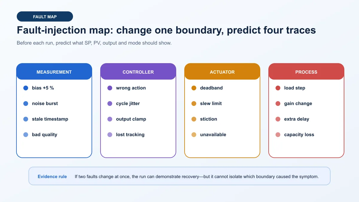
Design fault injection as an experiment

Measurement faults

Inject a known bias, repeatable noise burst, stale timestamp or bad-quality state. A bias changes the relationship between modeled truth and observed PV. Noise changes short-term variation. Staleness changes age without necessarily changing the number. Bad quality changes the state contract. Those faults should not be represented by the same Boolean because they lead to different diagnostic evidence and potentially different project responses.

Controller faults

Use wrong action, mismatched cycle, unexpected output clamp or lost tracking as controlled defects. Avoid publishing a “bad tuning value” as though it is universally bad; gains depend on algorithm form, units and plant. Instead save a known-good configuration and apply a declared relative change or a structural fault.

Actuator faults

Model deadband, slew limit, stiction and unavailable state separately. Deadband ignores small command changes. Slew limits the rate of applied movement. A simple stiction model can hold position until the command difference exceeds a threshold and then jump. Unavailable state prevents normal application and should be visible to the controller wrapper.

Process faults

Apply a load step, change process gain, add delay or reduce capacity. A capacity loss may pin output at its limit while PV remains short of SP; this is not automatically a controller failure. A delay increase can make an unchanged controller oscillatory or sluggish. The learner should locate the changed boundary before proposing a correction.

Translate the project to Siemens, Rockwell, Schneider or CLICK

Siemens PID projects

Current Siemens PID documentation covers technology objects and PID functions for supported S7-1200/S7-1500 environments, including documented process-value handling, controller modes, limits and commissioning behavior. Translate the project contract to the exact CPU, firmware and TIA Portal release. Record the technology-object or instruction version and its configured cycle. Do not copy screenshots or parameter values from a different revision and call that portability.

Rockwell Automation PID projects

Logix offers standard PID, Enhanced PID (PIDE) on supported controllers and newer PlantPAx process instructions for applicable platforms. Language availability and platform support differ; current Rockwell documentation notes, for example, that PIDE availability and replacement guidance depend on controller generation. Choose the instruction appropriate to the exact target and keep the vendor-neutral project evidence fields around it.

Schneider Electric PID projects

Machine Expert libraries include PID variants with documented timing, modes, manual control, anti-reset windup, bumpless transfer and error outputs. Some variants measure elapsed time while a fixed-cycle variant accepts a precise cycle. The project should assert which block/library/version it uses and test the documented enable, hold, manual and error behavior.

AutomationDirect CLICK PID projects

AutomationDirect publishes CLICK PID control help intended to support implementation in ladder logic. Use that current platform documentation for the specific CLICK family and software. Preserve the same project questions—units, timing, action, modes, limits, raw/applied output and test evidence—rather than forcing another vendor’s parameter names into the project.

Translation item	Vendor-neutral record	Platform-specific verification
algorithm form	position/velocity or declared form	exact instruction documentation
tuning units	gain, integral/derivative time or rate	field definitions and time base
execution	intended interval and measured behavior	supported task/call pattern
manual/track	applied-output alignment requirement	exact pins, modes and state behavior
limits/anti-windup	raw, limited and applied demand	internal/external limit integration
restart	desired effective mode and output	first-scan, prescan and retained-state rules
language/platform	project logic form	instruction availability on exact controller

Simulation, physical trainers and real plants

What simulation can prove

A deterministic browser or PLC simulator can prove the surrounding sequence behaves according to the implemented model: signal selection, mode transitions, timing assumptions inside the test environment, output constraints, fault injection, metrics and repeatable regression. It can teach the qualitative effects of gain changes and expose logic faults before hardware is available.

What simulation cannot prove

Simulation cannot certify real sensor accuracy, analog wiring, electrical protection, heater safety, motor starting, pump hydraulics, valve sizing, stiction magnitude, process gain, dead time, network scheduling, controller firmware behavior, independent protection or safe operating limits. It cannot authorize energization, bypasses, forcing or work on installed machinery.

A physical trainer is still an engineered system

Prefer a commercially designed low-energy trainer or an institutionally approved build. Document its energy sources and hazards. OSHA’s hazardous-energy rule addresses unexpected energization and stored energy in covered servicing work; site and jurisdiction requirements may be broader or different. Push buttons, software commands and PLC outputs are control functions, not energy-isolating devices.

Keep production OT access separate

Do not connect a learning simulator or unmanaged laptop to a production control network merely to obtain realistic tags. NIST’s OT security guidance emphasizes safety, reliability and performance alongside cybersecurity. Use an approved lab segment, controlled accounts, backups, change control, logging and recovery procedure. Remove or disable test pathways deliberately when the project ends.

Turn the project into credible portfolio evidence

Show the engineering decision, not only the interface

A strong portfolio entry contains a one-paragraph objective, simple architecture, I/O/state contract, process-model assumptions, test matrix, one normal trace, one failed or fault trace, calculated metrics, diagnosis and limitations. A video can demonstrate the run, but it does not replace the saved configuration and result table.

Include negative evidence

Show at least one test that failed for an understandable reason and what discriminating evidence led to the correction. “I increased Kp until it worked” is weaker than “output was saturated, so additional gain could not supply missing model capacity; the capacity-loss case remained a documented failure.” Negative evidence demonstrates troubleshooting judgment.

Make the result reproducible

Provide a version or commit identifier, simulator version, model parameters, controller interval, saved scenario and calculation sheet. If sharing project files would expose licensed vendor content or unsafe plant details, publish a sanitized evidence record and explain what was withheld.

Common PID project mistakes

Targeting an ambiguous keyword instead of a learner task

The unqualified singular “PID project” primarily means Project Initiation Document in current search results. A PLC page should use clear control-engineering wording and serve the plural project-idea task. Traffic from the wrong intent is not acquisition success.

Building hardware before proving the model and test harness

A physical rig adds wiring, protection, mechanics and safe-work demands before the learner knows whether scenarios reset or metrics calculate correctly. Prove the test harness in simulation first. Then justify which learning question truly requires hardware.

Tuning around scaling, direction or capacity defects

If PV and SP use different units, action is reversed, model updates are irregular or applied output is constrained, tuning changes obscure the cause. Pass static, manual-direction and authority checks before closed-loop optimization.

Showing only PV and SP

PV/SP traces can hide saturation, an inactive automatic mode, a downstream clamp or an unavailable actuator. Include raw, limited and applied output plus effective mode and quality.

Changing several variables in one run

Changing tuning, filter, model delay and disturbance simultaneously prevents attribution. A recovery demonstration may intentionally combine failures, but a diagnostic experiment should change one boundary.

Treating one vendor’s gain units as universal

Parallel, ideal, dependent and independent forms are not interchangeable. Integral can be a gain, time or repeats per unit time. Derivative may act on error or measurement. Record the exact block and units.

Claiming the simulator validates a real plant

A model demonstrates behavior under its assumptions. Real process commissioning must prove sensors, actuators, timing, capacity, modes, independent protection and operating limits under approved procedures.

Diagnostic answer map for PID project search and AI assistants

Natural-language query	Concise answer	Boundary to preserve
What is a good PID control project for PLC training?	Start with a virtual thermal chamber using temperature PV, bounded heater demand, heat-loss disturbance and tests for modes, limits and quality.	It teaches the method; it is not a real heater design.
Which PID project is easiest for a beginner?	A slow virtual temperature loop is easier to observe and reset than fast flow, pressure or motion.	Easy does not mean a universal tuning recipe.
What must a PLC PID project include?	Requirement, signal/state contract, repeatable model, documented controller, scenarios, metrics, fault tests, evidence and a transfer boundary.	A working block or one trend is incomplete.
How do I test setpoint tracking?	Start from a saved baseline, apply a defined SP change and calculate overshoot, settling, final error, saturation and output movement.	Do not change the plant or limits during comparison.
How do I test disturbance rejection?	Hold SP constant, apply one recorded load change and measure deviation, recovery and output response.	This is a different objective from SP tracking.
What faults should a PID project inject?	Bias, noise, stale/bad PV, wrong action, timing mismatch, limit, lost tracking, deadband, stiction, load, delay and capacity loss.	Inject one boundary at a time for diagnosis.
Can tuning fix an undersized actuator?	No. When applied output is at its limit and capacity is insufficient, gains cannot create authority.	Prove command, feedback and process response first.
Can a browser simulator validate PLC PID logic?	It can validate the implemented model, sequence, modes, limits, metrics and regression behavior.	It cannot certify exact hardware or a real process.
What should I show in a PID project portfolio?	Objective, architecture, assumptions, test matrix, normal/fault trends, metrics, decision, version and limitations.	Sanitize licensed or plant-sensitive information.
How do I move from simulation to hardware?	Use an approved design and trainer, verify exact manuals, hazards, I/O, protection, isolation, commissioning and recovery under qualified supervision.	Simulation is not authorization to energize.

Frequently asked questions

What is the best first PID project for a PLC beginner?

A virtual temperature-control chamber is the best first project because its slow response makes delay, overshoot, settling, output saturation and heat-loss disturbances easy to observe. Use a bounded heater model and explicit sensor quality. Complete manual-direction, mode-transfer, setpoint, disturbance, limit and fault tests before considering physical hardware.

Is “PID project” the same as a Project Initiation Document?

It can be. The current singular search intent is dominated by the project-management meaning “Project Initiation Document.” This page deliberately uses the plural phrase “PID projects” for proportional-integral-derivative control learning projects and does not claim the unrelated project-management traffic.

What signals should I trend in a PLC PID project?

Trend setpoint, raw and validated process variable, measurement quality or age, raw PID request, limited output, applied output, requested and effective mode, active constraint and actuator feedback when available. Synchronized timestamps and a named scenario are essential for diagnosis.

How do I calculate whether a PID project passed?

Predeclare a response band and calculate metrics such as peak overshoot, settling time, mean final error, integrated absolute error, time at output limits and output movement. Also require correct modes, quality handling and recovery. Use the same initial state, model, stimulus and observation window for comparisons.

Should a PID project use real hardware?

Not initially. A deterministic simulator is usually the better first environment because it can reset, repeat and inject faults without real energy. Use physical hardware only when the learning objective requires it and an approved design, hazard assessment, exact documentation, qualified supervision and safe-work process are in place.

How do I test anti-windup in a PID project?

Deliberately constrain applied output while error persists, trend raw and applied output plus the controller’s integral or limit status, then remove the constraint under controlled conditions. Pass criteria should limit recovery delay and overshoot. Use the exact platform’s documented anti-windup and tracking behavior.

What is the difference between a PID program and a PID project?

A PID program is the reusable controller implementation around one function block: timing, scaling, modes, tracking, limits, diagnostics and commissioning behavior. A PID project adds a selected process model, learning question, disturbances, fault injections, response metrics, test matrix and portfolio evidence.

Can one PID project teach temperature, flow, pressure and level control?

One framework can organize all four, but the process dynamics and constraints are different. Temperature is slow and lagged, level accumulates flow imbalance, and flow or pressure can respond much faster and show different noise and capacity effects. Keep separate saved models and acceptance criteria.

What makes a PID project useful for troubleshooting practice?

It must expose raw, limited and applied output, quality, mode, feedback and a known-good baseline, then inject one controlled measurement, controller, actuator or process fault. The learner should identify the first evidence divergence and propose a discriminating next test before changing tuning.

Can a PID simulator prove my real tuning values are safe?

No. Simulator results apply to the implemented model and assumptions. Real tuning depends on actual sensors, actuators, process gain, delay, nonlinearities, constraints, interactions, protection and operating limits. Transfer only through the approved commissioning and change process.

Sources, review scope, and limitations

This guide was reviewed on August 29, 2026. Product support, firmware, programming software, instruction behavior and standards change. Verify the exact installed platform and current source before implementation.

• SIMATIC S7-1200/S7-1500 PID control function manual, November 2025 — Siemens
• Enhanced PID (PIDE), Logix Designer 38.02 — Rockwell Automation
• Proportional Integral Derivative (PID), Logix Designer 38.01 — Rockwell Automation
• Anti-reset windup and bumpless transfer for PID — Rockwell Automation
• Timing modes in Logix Designer — Rockwell Automation
• PID function block — Schneider Electric Machine Expert
• FB_PID function block — Schneider Electric Machine Expert
• ControlLoopLibrary documentation — Schneider Electric
• PID Control in CLICK — AutomationDirect
• The PID Controller and Theory Explained — National Instruments
• PID tuning algorithm and objectives — MathWorks
• PID tuning for setpoint tracking versus disturbance rejection — MathWorks
• Anti-windup control using a PID Controller block — MathWorks
• IEC 61131-3:2025 programmable-controller programming languages — IEC
• ISA-TR5.9-2023 PID algorithms and performance listing — ISA
• ANSI/ISA-5.1-2024 instrumentation and control symbols scope — ISA
• 29 CFR 1910.147 control of hazardous energy — OSHA
• NIST SP 800-82 Rev. 3 Guide to Operational Technology Security — NIST

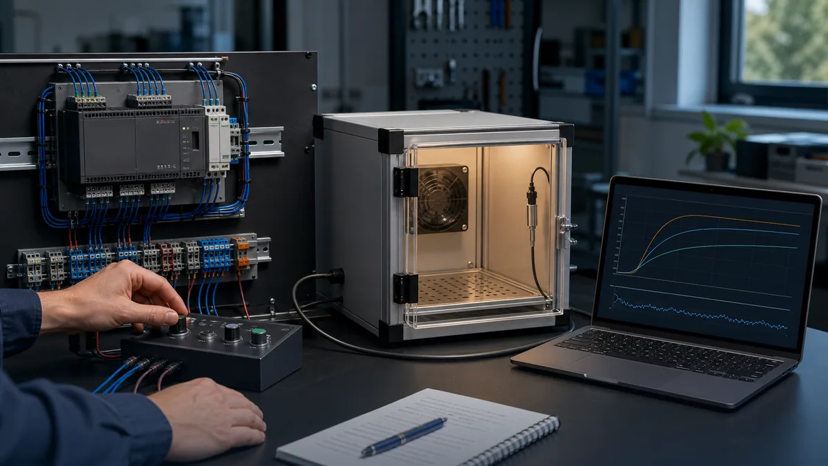
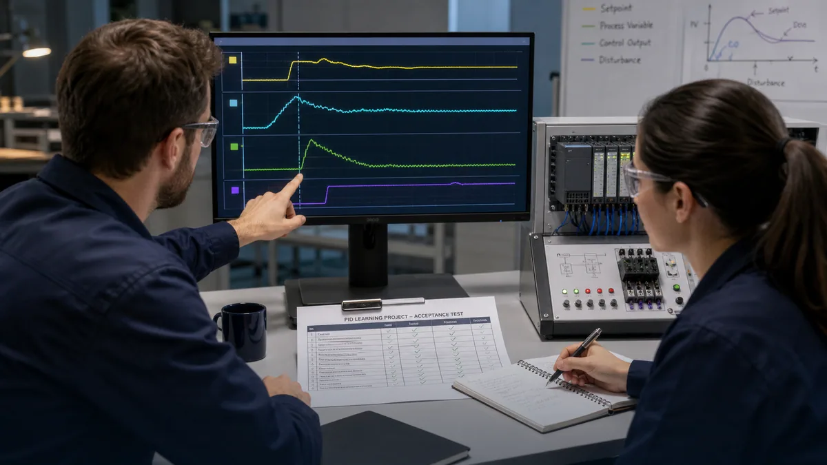
The eight projects, models, tag names, numerical examples, test cases and acceptance examples are original editorial teaching designs. They are not vendor code, field wiring, P&IDs, safety functions, equipment specifications, tuning prescriptions or operating procedures. The generated scenes are contextual illustrations; the remaining figures are deterministic explainers.

This page does not authorize connecting, energizing, operating, forcing, bypassing, tuning or testing installed equipment. Qualified and authorized personnel must apply the site hazard assessment, energy-control and electrical safe-work rules, exact manufacturer documentation, process and equipment limits, independent protection, cybersecurity controls, management of change and approved commissioning/recovery procedures.