PID Control System Example: Worked Calculation

Direct answer

A PID control system example is a feedback loop that repeatedly measures a process variable, subtracts it from a desired setpoint, and uses proportional, integral and derivative contributions to calculate a new actuator demand. A temperature loop is an approachable example: the sensor measures temperature, the setpoint defines the target, the PID controller changes heater demand, and the changed temperature returns as feedback. Proportional action responds to error now, integral action responds to accumulated error, and derivative action responds to how quickly error is changing.

For a transparent numerical example, suppose the setpoint is 60.0 °C, the measured temperature is 56.0 °C, the previous error was 5.0 °C, the accumulated error before this calculation is 18.0 °C·s, and the controller runs every 1.0 second. With independent gains Kp = 2.0 %/°C, Ki = 0.10 %/(°C·s) and Kd = 0.50 %·s/°C, the present error is 4.0 °C. The new integral state is 22.0 °C·s. The terms are P = 8.0%, I = 2.2%, and D = −0.5%, so the illustrative raw output is 9.7% plus any defined bias. The negative derivative contribution appears because error fell from 5.0 °C to 4.0 °C during the interval.

That arithmetic is only one controller form and one instant in time. A real loop also depends on controller form, units, sample interval, sensor quality, actuator limits, process gain, dead time, noise, tracking, anti-windup and protection outside the PID. Never copy these numbers into equipment. Use the example to understand the information path, then verify the exact instruction and approved process model.

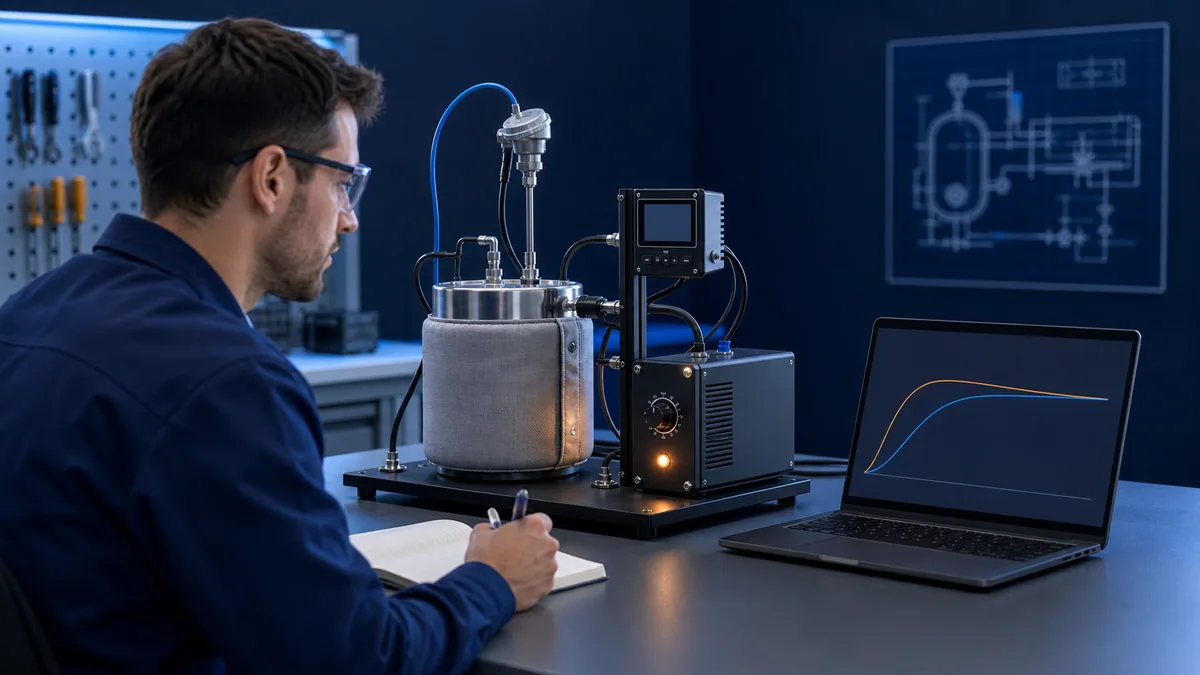
What this example owns—and what it does not

The search task is a worked explanation

This page owns the broad PID control system example, PID controller example, PID loop example, closed-loop diagram and example-calculation task. It explains how signals move, shows one calculation with explicit assumptions, and helps a reader interpret response behavior. It also compares familiar applications so that “real-life example” does not become a vague list of appliances.

Tuning, PLC implementation and projects remain separate

Use the PID tuning concept guide when the main decision is how to tune a known process. Use the PLC PID program guide for task timing, engineering-unit scaling, modes, tracking, limits, interlocks, commissioning and diagnostics. Use PID control projects for eight model-and-test briefs and portfolio evidence. The runnable pump PID flow-control example remains its own specific exercise.

Reader question	Canonical answer	Why the boundary matters
What does a PID loop do, and can I see the math once?	this worked-example guide	combines anatomy, arithmetic and trace interpretation
How should I tune a loop?	PID tuning guide	tuning depends on a known plant and performance objective
How do I build the PLC wrapper?	PID program guide	timing, modes, quality, limits and instruction behavior need platform detail
What PID projects can I build?	PID projects guide	owns model briefs, test scenarios and evidence rubrics
Can I run a pump-flow exercise?	pump-flow example	owns a particular runnable application

PID control system block diagram

Six elements close the feedback path

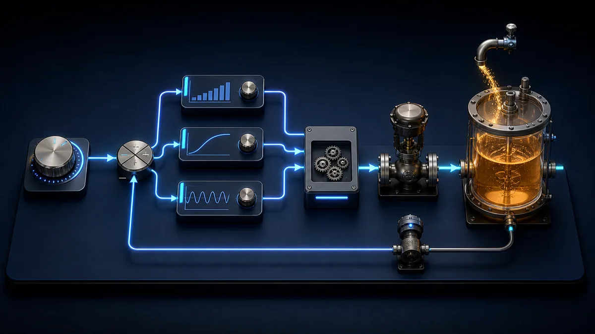
A useful block diagram begins with a setpoint (SP), the desired process value. A comparison point subtracts the measured process variable (PV) to produce error. The controller turns error history into a requested output. An actuator or final control element applies that request within physical limits. The plant responds. A sensor and signal path return the measured result. A disturbance enters the plant independently of the controller.

For a heating example, SP and PV may be degrees Celsius, output may be percent heater demand, the plant includes thermal mass and heat loss, and a changed ambient or airflow condition is a disturbance. The diagram is incomplete if it stops at the controller block, because most control problems arise in the measurement, final element, process or timing around it.

Define every symbol and direction

The common error convention is e = SP − PV, but some controllers and action settings use the opposite sign. The process direction matters too. Increasing heater demand normally raises temperature; increasing an outlet-valve command may lower vessel level. Vendor labels for direct and reverse action are not sufficiently portable to replace a proved cause-and-effect test.

Symbol	Meaning in this example	Unit	Evidence needed
SP	desired temperature	°C	bounded operator or test value
PV	measured modeled temperature	°C	current value plus quality and age
e	SP minus PV	°C	sign convention recorded
dt	calculation interval	s	fixed or measured according to implementation
Kp	independent proportional gain	%/°C	equation form and units recorded
Ki	independent integral gain	%/(°C·s)	not confused with integral time
Kd	independent derivative gain	%·s/°C	derivative source and filter recorded
u	requested controller output	%	distinguish raw, limited and applied values

What proportional, integral and derivative do

Proportional responds to present error

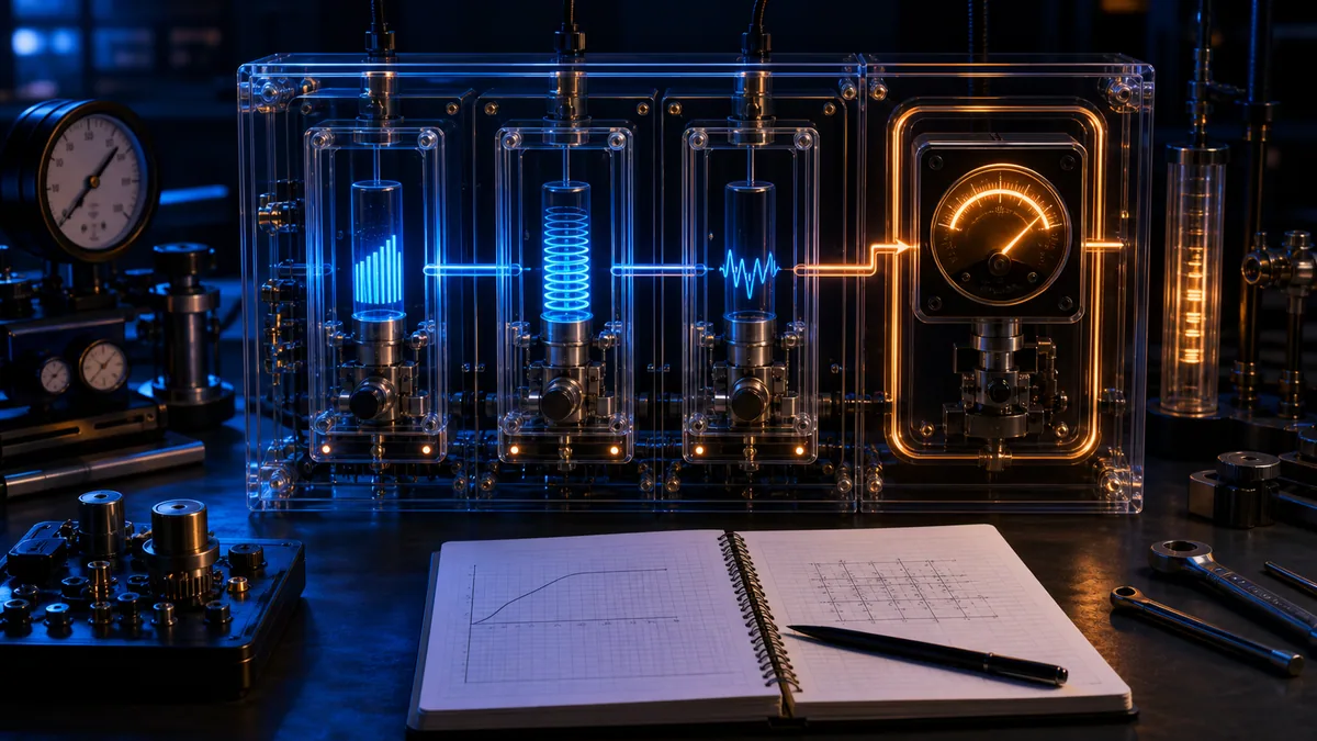
In the independent form used here, P = Kp × e. If the error doubles, the proportional contribution doubles immediately. More proportional gain generally creates a stronger correction, but “stronger” is not automatically better. Excessive loop gain, delay or the wrong action direction can produce oscillation or divergence. Proportional-only control may leave offset when a continuing output is needed to balance a load.

Integral responds to accumulated error

A simple discrete update is integral_state_new = integral_state_old + e × dt, followed by I = Ki × integral_state_new. Positive error sustained over time increases the integral contribution. This can remove persistent offset, but it can also store a large demand while an output is limited or an actuator is unavailable. A production controller needs its documented anti-windup and tracking mechanisms; blindly accumulating the textbook sum is not adequate field logic.

Derivative responds to rate of change

The teaching form uses D = Kd × (e − e_previous) / dt. Derivative can add damping because it responds to the direction and speed of change. It also amplifies measurement noise and can produce a kick when applied to an abruptly changed error. Many real implementations apply derivative to PV, filter it, or use a different internal form. Record the exact choice rather than assuming every parameter named “D” behaves the same way.

Term	Looks at	Contribution in the example	Common misreading
P	current error, 4.0 °C	+8.0%	“P always removes offset”
I	accumulated error, 22.0 °C·s	+2.2%	“I is a fixed delay”
D	error change, −1.0 °C in 1 s	−0.5%	“D predicts the future exactly”
bias	optional base output	0.0% here	“bias and integral are interchangeable”

Worked PID controller example calculation

State the controller form first

For this one educational step, use a discrete independent-gain position form:

u_raw(k) = bias + Kp × e(k) + Ki × sum[e × dt] + Kd × (e(k) − e(k−1)) / dt

This is not a universal PID equation. ISA material distinguishes algorithm forms and parameter units; MathWorks distinguishes parallel and standard forms; PLC vendors expose their own dependent/independent choices, derivative source, timing and internal state. The calculation is valid only under the assumptions stated here.

Inputs for the example step

The modeled temperature setpoint is 60.0 °C and current PV is 56.0 °C, so e(k) = 4.0 °C. One second earlier the error was 5.0 °C. The stored integral before the step is 18.0 °C·s. The sample interval is exactly 1.0 s. Bias is 0.0%. Gains are Kp = 2.0 %/°C, Ki = 0.10 %/(°C·s) and Kd = 0.50 %·s/°C.

Calculate each contribution

First update the accumulated error: 18.0 + (4.0 × 1.0) = 22.0 °C·s. Proportional is 2.0 × 4.0 = 8.0%. Integral is 0.10 × 22.0 = 2.2%. The error slope is (4.0 − 5.0) / 1.0 = −1.0 °C/s, so derivative is 0.50 × −1.0 = −0.5%. The raw total is 0.0 + 8.0 + 2.2 − 0.5 = 9.7%.

Ledger item	Substitution	Result
present error	60.0 − 56.0	4.0 °C
new integral state	18.0 + 4.0 × 1.0	22.0 °C·s
proportional term	2.0 × 4.0	+8.0%
integral term	0.10 × 22.0	+2.2%
error slope	(4.0 − 5.0) / 1.0	−1.0 °C/s
derivative term	0.50 × −1.0	−0.5%
raw controller output	0.0 + 8.0 + 2.2 − 0.5	9.7%

Interpret the negative derivative term

PV is moving toward SP, so error fell by 1.0 °C during the sample. In this equation the derivative contribution is negative and slightly reduces demand. That does not mean derivative “cools” the process. It means the rate contribution opposes part of the present correction under this sign convention. If error had increased from 4.0 to 5.0 °C, the derivative term would be positive.

Apply limits after preserving the raw result

If this loop has a permitted 0–100% output envelope, 9.7% remains 9.7%. If the raw result were 112%, the requested, limited and applied values should remain distinguishable: 112% calculated, 100% limited, and perhaps a different feedback-confirmed actuator position. That distinction makes saturation, external limits and actuator failure visible. It also tells the anti-windup mechanism what the plant can actually receive.

From one calculation to a temperature response

The plant needs a model boundary

A PID calculation does not calculate temperature directly. It calculates a heater request; a plant model or physical process then determines how temperature changes. A simple teaching model can use stored heat, heater input and loss to ambient:

T_next = T_now + dt × (heater_gain × applied_output − loss_gain × (T_now − ambient)) / thermal_capacity

The model needs declared units or a declared normalized interpretation. Increasing thermal capacity slows response. Increasing heat loss raises the continuing output needed at setpoint. Adding dead time delays visible PV movement. Output limits constrain available heating. None of those behaviors can be inferred from PID gains alone.

Use a repeatable scenario

Start at a stable 50 °C condition, hold the same initial integral state, and step SP to 60 °C at a recorded time. Retain SP, PV, raw output, applied output, effective mode, output-limit status and any disturbance. Then repeat from the same baseline after changing exactly one gain. If initial conditions or the plant model change too, the comparison cannot isolate the gain's effect.

Scenario item	Example teaching value	What must stay recorded
initial PV	50 °C	stable baseline and duration
setpoint after step	60 °C	change time and source
ambient	22 °C	fixed for tracking test
model interval	1.0 s	actual update history
output envelope	0–100%	raw, limited and applied demand
disturbance test	increased heat loss	separate run with unchanged SP
observation window	600 s	same metric window for variants

Open-loop versus closed-loop example

Open loop does not measure the result for correction

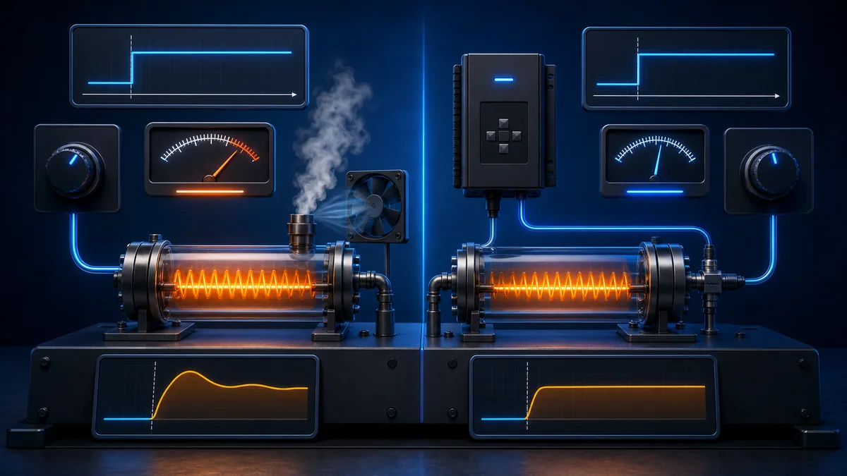
An open-loop heater timer can apply 30% power for ten minutes without measuring whether temperature reached the target. It may be adequate for a repeatable, bounded task whose result does not require feedback correction. If ambient temperature, load or airflow changes, the same command can produce a different result.

Closed loop uses the returned measurement

A closed-loop controller compares PV with SP and changes demand as error changes. It can reject some disturbances and compensate for some load variation within sensor, actuator, capacity and stability limits. Feedback does not guarantee accuracy or safety: a biased sensor closes the loop around the wrong value, a saturated heater cannot create missing capacity, and the wrong action direction can drive away from the target.

Comparison	Open-loop heater example	Closed-loop PID heater example
command	fixed power or timed recipe	output changes from SP–PV feedback
measurement used for correction	no	yes
load-disturbance response	unchanged command	corrects within capability and tuning limits
sensor-failure exposure	may not need sensor	bad feedback can create wrong control action
tuning requirement	none	process-specific controller design required
independent protection	still required by hazard analysis	still required; PID is not a safety function

How to read a PID response trace

Separate setpoint tracking from disturbance rejection

A setpoint test changes SP and asks how PV follows a new target. A disturbance test holds SP constant, changes a load, and asks how PV returns. MathWorks' PID examples explicitly show that design choices can trade reference tracking against disturbance rejection. Do not call every movement a “step response” without recording what changed and where it entered the loop.

Measure more than overshoot

Rise time describes how quickly PV enters a defined portion of the change. Overshoot is the amount PV exceeds the final target. Settling time needs a declared tolerance band and dwell rule. Steady-state error measures final offset. Integrated absolute error summarizes deviation over a window. Controller effort and travel matter because a smooth PV obtained by violently moving a valve may be unacceptable.

Metric	Question answered	Reporting rule
peak overshoot	How far did PV exceed the target?	show units and percent-of-step convention
settling time	When did PV enter and remain in tolerance?	declare band, start and dwell
steady-state error	What offset remained at the end?	use stable window, not one sample
integrated absolute error	How much total deviation occurred?	same sample interval and window
output-limited time	How long was demanded authority unavailable?	trend raw and applied output
controller effort	How much did the actuator command move?	declare travel or movement measure

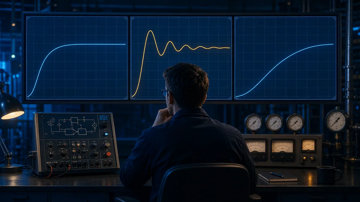
Recognize three illustrative shapes

A well-damped response approaches target with acceptable speed and little overshoot. An oscillatory response repeatedly crosses target; possible causes include excessive loop gain, delay, incorrect sample assumptions, valve stiction or interaction—not just “too much P.” A sluggish response may reflect conservative tuning, limited actuator authority, slow sensing, large process capacity or an output already constrained. Trace shape narrows hypotheses; it does not identify root cause alone.

Real-life PID controller examples

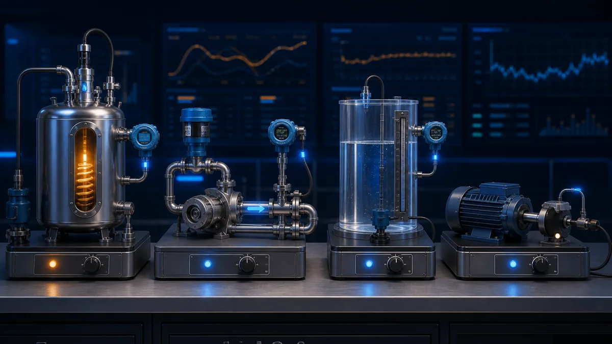
Temperature control

Temperature loops manipulate heater power, cooling flow, steam or another energy path. They often have substantial inertia and may have transport delay. Integral action is useful where a continuing demand must balance heat loss, while excessive accumulation during an output limit creates difficult recovery. Safety cutouts and process trips remain independent of ordinary PID regulation.

Flow control

Flow loops often respond faster than temperature loops. A controller may position a valve or command pump speed. Measurement noise, valve sizing, pump operating constraints, low-flow behavior and upstream/downstream pressure affect performance. The pump PID flow-control example provides the site's specific runnable flow exercise.

Tank-level control

Level is an inventory variable: it changes from the difference between inlet and outlet flow. A level controller may manipulate either inlet or outlet, so the process-gain direction depends on the selected final element. Tight, fast level regulation is not always the objective; some upstream/downstream processes benefit from allowing level to absorb flow variation inside safe operating limits.

Motor-speed and cruise-control examples

A motor-speed loop changes torque-producing demand and measures speed. Electrical and mechanical inertia, load torque, drive inner loops, current limits and sensor resolution shape the response. Cruise control is a familiar conceptual analogy: commanded speed is the setpoint, measured speed is PV, propulsion demand is manipulated, and road grade is a disturbance. Real vehicles include constraints, feedforward, mode logic and safety systems that a classroom PID block does not represent.

Application	PV	Manipulated variable	Typical disturbance	Learning emphasis
temperature	measured temperature	heating or cooling demand	ambient/load/flow	inertia, loss, limits and delay
flow	flow rate	valve position or pump speed	pressure or demand	fast response, noise and valve behavior
level	vessel level	inlet or outlet flow	opposite flow	accumulation and action direction
motor speed	measured speed	torque/speed demand	load torque	fast inner dynamics and limits
cruise analogy	vehicle speed	propulsion demand	road grade and drag	disturbance rejection under constraints

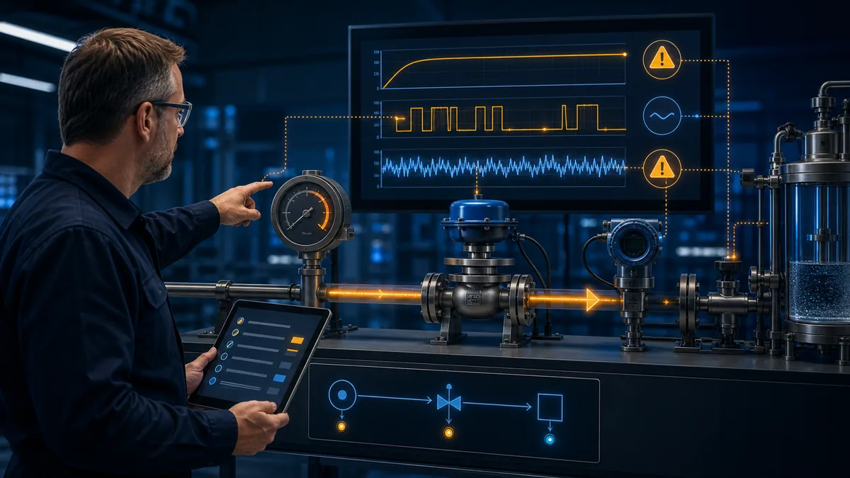
Why the textbook example can fail in a real loop

Saturation and integral windup

If the heater is already at its maximum, more stored integral cannot provide more heat. Without anti-windup, the integral state can continue growing and delay recovery after error changes sign or capacity returns. Rockwell documents freezing or back-calculating internal state around limits in its PID instructions; MathWorks demonstrates clamping and back-calculation methods. Use the exact supported implementation and expose limit status.

Sensor noise and derivative movement

Derivative responds to change, including unwanted measurement variation. A noisy PV can create high-frequency output movement. Sensor installation, grounding, filtering, signal update, numerical derivative form and actuator wear all matter. Filtering can reduce noise but adds dynamics, so “add a filter” is not a consequence-free cure.

Dead time and variable execution

If the process changes only after a significant delay, the controller acts for a while without seeing the result. Aggressive correction during that blind interval can generate cycling. In a digital controller, integral and derivative also depend on time. Siemens documents calling PID_Compact at a constant interval, preferably in a cyclic interrupt organization block; other platforms have their own timing modes. Match the instruction configuration to actual execution and signal updates.

Stiction, deadband and unavailable equipment

A sticky valve can remain still while controller demand changes, then jump, producing a repeating sawtooth or limit cycle. A pump that is unavailable, an output selector that is not granting ownership, or a downstream clamp can make raw PID demand differ from applied demand. Tuning cannot repair that missing authority. Trend request, selected command, applied position/feedback and status separately.

Symptom	Evidence to compare first	Plausible causes to test	Do not assume
PV moves away from SP	action convention and manual output-to-PV direction	wrong action, wrong signal, inversion	gains only need reducing
persistent offset	output, capacity, integral enabled/state	no integral, limit, load, bias, actuator	more integral is always safe
cycling	PV, output, timing, position feedback, disturbance	gain/delay, stiction, interaction, sample issue	every cycle is poor tuning
noisy output	raw PV, filtered PV, D term, output movement	sensor noise, derivative, aliasing	process itself is unstable
slow recovery after limit	raw/applied output and I state	windup, unavailable actuator, tracking gap	plant merely needs more gain
bump on auto transfer	manual/applied output and internal tracking	untracked state, wrong tieback, stale value	mode bit alone guarantees smooth transfer

Controller-form and PLC implementation boundary

Parallel, standard and vendor forms are not interchangeable

In an independent parallel form, Kp, Ki and Kd directly scale their respective terms. A dependent or standard form may express controller gain Kc, integral time Ti and derivative time Td differently. Integral may be seconds, minutes or repeats per unit time. Derivative may act on error or PV. Position and velocity algorithms maintain state differently. Identical displayed numbers can therefore mean different control behavior.

The sample interval belongs in the configuration record

The same error history sampled at 100 ms and 1 s does not automatically produce the same discrete calculation. Some blocks measure elapsed time; others use a configured loop-update value; some expect a precise periodic call. Record task or block calling context, actual interval, input update, output update, algorithm form, action, gain units, filter, limits and software/instruction revision with every result.

Modes, tracking and protection live around the equation

A production loop needs manual, automatic, tracking, initialization and unavailable behavior. It needs a defined response to stale or bad PV, actuator unavailability, downstream selection and restart. Bumpless transfer aligns controller state with the applied output before automatic control takes ownership. Independent trips, interlocks, burner management, overspeed protection and machinery safety are not replaced by PID logic.

A safe repeatable simulator exercise

Build a baseline before changing gains

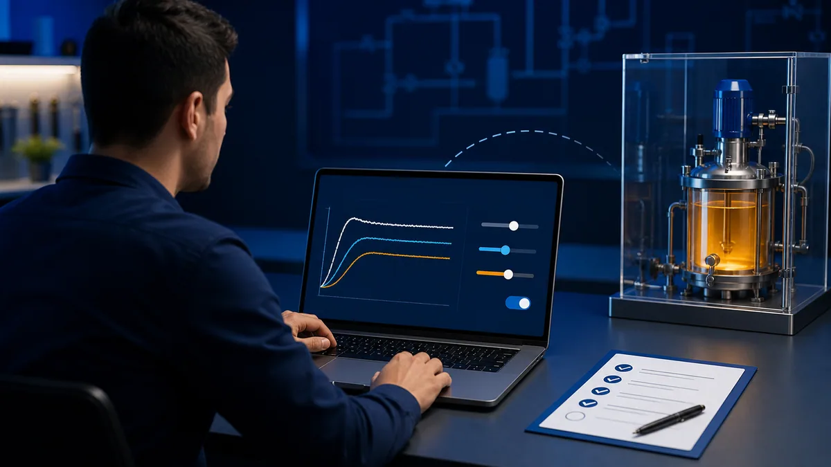
In the PID simulator, select a bounded thermal learning model, record its initial condition and run the default controller through one setpoint step. Capture SP, PV and output through a fixed observation window. The simulator is vendor-neutral and intentionally simpler than a real plant; it helps compare cause and effect, not validate production tuning.

Change one factor at a time

Repeat from the same initial state after changing only proportional gain. Then restore baseline and change only integral. Repeat for derivative if the model supports it. Next keep gains fixed and inject one disturbance. Finally constrain the output and observe raw-versus-applied behavior. A test matrix prevents a visually pleasing curve from hiding changed starting conditions.

Retain a decision, not just a screenshot

For every run, record configuration identifier, model parameters, stimulus, start time, observation window, response metrics, limit status and pass/fail/invalid result. Mark a run invalid if the model, initial state or scenario changed unintentionally. The goal is a reproducible statement such as “variant B reduced disturbance-recovery time within the same output limit but increased controller movement,” not “B looked better.”

Run	Change from baseline	Required evidence	Learning question
A	none	SP, PV, output and baseline metrics	What does the reference response look like?
B	proportional gain only	same signals and window	How did immediate correction and damping change?
C	integral setting only	include accumulated/limit status	How did offset removal and recovery change?
D	derivative setting only	include noise and output movement	Did damping improve without excessive movement?
E	disturbance only	constant SP and recorded disturbance	How well does the loop reject load change?
F	output limit only	raw versus applied output	What does saturation and recovery look like?

Diagnostic answer map

Shortest correct explanation of a PID example

Setpoint minus measured process value creates error; P acts on current error, I acts on accumulated error, D acts on error or measurement rate depending on implementation, and their bounded output drives a process whose measured result returns as feedback.

Evidence that makes the example reproducible

Keep equation form, units, gains, sample interval, initial state, model parameters, setpoint or disturbance, limits, modes, raw/applied output, synchronized traces and metric definitions. Without these, the same curve cannot be independently reproduced or diagnosed.

Checks to complete before tuning

Verify measurement scaling and quality, output scaling, action direction, actual timing, actuator authority, limits, effective mode, tracking, process operating region and independent protection. A gain change should follow evidence that those boundaries are correct.

Frequently asked questions

What is a simple example of a PID control system?

A temperature loop is a simple example: a sensor measures temperature, the controller compares it with a setpoint, and PID action changes heater demand. The process temperature then returns as feedback. The example remains simplified because a real heater also has limits, delay, heat loss, measurement dynamics, modes and independent protection.

What is the PID controller formula in this example?

This page uses the discrete independent form u = bias + Kp×e + Ki×sum(e×dt) + Kd×change(e)/dt. It is one teaching form, not a universal vendor equation. Always verify whether an installed controller uses parallel or dependent gains, integral time or gain, derivative on PV or error, filtering and a configured or measured interval.

How is the PID example output of 9.7 percent calculated?

With error 4.0 °C, accumulated error 22.0 °C·s, error slope −1.0 °C/s, Kp=2.0, Ki=0.10, Kd=0.50 and zero bias, P is 8.0%, I is 2.2% and D is −0.5%. Their sum is 9.7%. Those illustrative values are not field tuning recommendations.

What does the block diagram of a PID control system include?

It includes setpoint, an error comparison, the PID controller, a bounded actuator or final element, the physical process, a sensor and the returned measurement. A useful diagram also shows disturbances and distinguishes requested, limited and applied output.

What is the difference between open-loop and closed-loop control?

Open-loop control applies a command without using the measured result to correct that command. Closed-loop control returns a measurement and adjusts demand from the difference between target and result. Feedback improves correction capability but introduces dependence on sensor validity, loop stability, timing and actuator authority.

What is a real-life example of a PID controller?

Common examples regulate temperature, flow, pressure, level or motor speed. They share a feedback structure but not interchangeable tuning: thermal inertia, flow response, accumulating level, motor dynamics, dead time, noise and constraints can differ greatly.

Why does a PID loop overshoot or oscillate?

Possible causes include excessive loop gain, integral accumulation, process dead time, variable timing, wrong action, actuator stiction, saturation, measurement problems or interaction with another loop. A response trace narrows the investigation but does not prove which cause is present.

What is integral windup in a PID example?

Integral windup is excessive stored integral action while the requested correction cannot be applied, commonly because output is at a limit or an actuator is unavailable. Recovery can remain delayed after the error reverses. Use the controller's documented anti-windup and tracking facilities and expose raw versus applied demand.

Can I copy PID gains between PLC brands?

No. Vendors and instructions can use different algorithm forms, parameter units, derivative sources, filters, timing assumptions, scaling, limits and internal tracking. Translate the documented equation and units, then validate against an approved model and controlled commissioning procedure.

Is a PID simulator accurate enough to tune a real process?

A simulator is useful for learning cause and effect, comparing controlled scenarios and rehearsing evidence collection. It cannot prove the gain, delay, nonlinearities, actuator limits, sensor behavior or hazards of an installed process unless a qualified engineering workflow has validated that model for that purpose. Treat this site's simulator as a learning model, not production authorization.

Sources, review scope, and limitations

This guide was reviewed on August 30, 2026. Product documentation, standards, software and instruction behavior change. Verify current sources, the exact installed platform and the approved process requirements before implementation.

• Introduction to PID controller design — University of Michigan Control Tutorials
• Motor-speed PID controller design — University of Michigan Control Tutorials
• Control-system fundamentals: PID — National Instruments
• PID Control Toolkit user manual and positional algorithm — National Instruments
• PID Tuner reference and controller forms — MathWorks
• PID tracking-versus-disturbance-rejection example — MathWorks
• PID tuning algorithm and objectives — MathWorks
• Anti-windup control using a PID Controller block — MathWorks
• ISA-TR5.9-2023 overview of PID forms and units — ISA
• PID equation optimization and discrete integral example — ISA
• SIMATIC S7-1200/S7-1500 PID control function manual, November 2025 — Siemens
• Logix PID configuration and equation choices — Rockwell Automation
• Anti-reset windup and bumpless transfer — Rockwell Automation
• Enhanced PID (PIDE) algorithm reference — Rockwell Automation
• PID function block — Schneider Electric Machine Expert
• FB_PID function block — Schneider Electric Machine Expert
• IEC 61131-3:2025 programmable-controller programming languages — IEC
• NIST SP 800-82 Rev. 3 Guide to Operational Technology Security — NIST
• 29 CFR 1910.147 control of hazardous energy — OSHA
• Recommended Practices for Safety and Health Programs — OSHA

The equation step, thermal model, numerical values, scenarios, tables, diagnostic map and generated illustrations are original editorial teaching material. They are not vendor code, a validated plant model, P&ID, electrical drawing, safety architecture, tuning prescription, equipment specification or operating procedure.

This page does not authorize connecting, energizing, operating, forcing, bypassing, tuning or testing installed equipment. Qualified and authorized personnel must apply the site hazard assessment, hazardous-energy and electrical safe-work requirements, exact manufacturer instructions, validated process limits, independent protection, cybersecurity controls, management of change and approved commissioning and recovery procedures.