PLC Analog I/O Signals: 4–20 mA, Voltage and Diagnostics

Direct answer

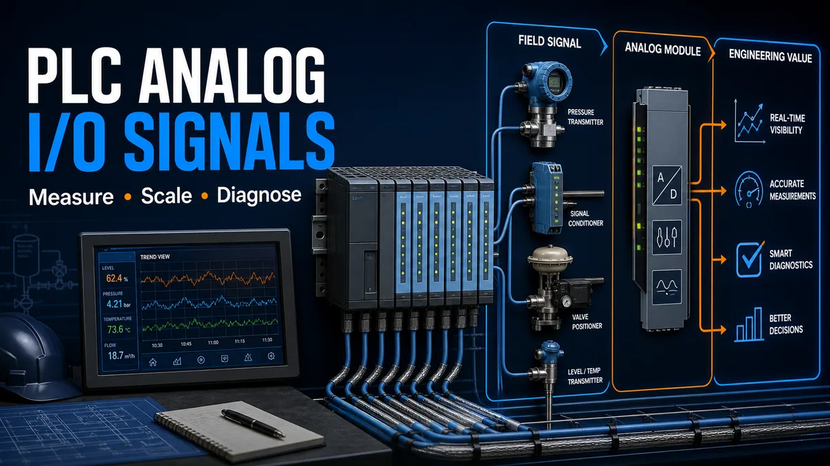
A PLC analog input converts a continuous electrical signal—such as 4–20 mA, 0–10 V, ±10 V, thermocouple voltage or RTD resistance—into digital channel data plus status. The program validates channel quality, maps the usable raw or electrical span into engineering units, applies only the filtering the process can tolerate, and keeps bad-quality behavior separate from numerical clamping. A PLC analog output performs the reverse path: a bounded engineering command becomes module data and then a current or voltage signal for a positioner, drive or other receiving device.

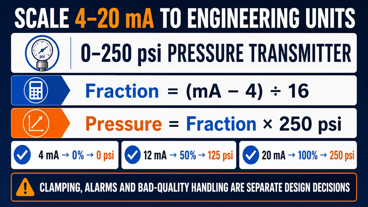
For a 4–20 mA pressure transmitter scaled 0–250 psi, the ideal fraction of span is (measured mA − 4 mA) ÷ 16 mA. At 12 mA, the fraction is 0.5, so the ideal pressure is 125 psi. That arithmetic is only one layer. The channel range must match the physical circuit; transmitter and input must have enough loop voltage; module diagnostics must be evaluated; and accuracy, resolution, isolation, common mode, noise, update time and fail behavior must meet the real application.

Do not infer a valid measurement from a plausible number alone. A module can retain a last value, substitute a fault value, saturate at a limit or report a raw code while the channel quality is bad. Preserve the raw value, configured range and diagnostic status together.

For a PLC analog output example, assume an approved module maps a documented raw range of 0…27648 to a configured 4…20 mA channel and the application requests 62.5%. The bounded fraction is 0.625, the illustrative raw command is 17280, and the ideal measured current is 14 mA. Those numbers are valid only for that stated mapping. The real acceptance chain is requested engineering command → bounded/rate-limited command → module data and status → measured current or voltage → receiving-device indication → actuator and process response.

Establish the safety and measurement boundary

A displayed value is not an electrically safe state

Opening an enclosure, lifting a conductor, inserting a meter, applying a loop calibrator or changing an output can expose electrical, pressure, temperature, chemical and machine-motion hazards. OSHA's hazardous-energy rule states that push buttons, selectors and control-circuit devices are not energy-isolating devices. A PLC in program mode, a zero output command or an HMI showing 0% does not establish isolation.

Follow the site-specific energy-control and electrical safe-work procedures. Qualified, authorized people must determine when equipment is de-energized and verified, when process pressure or stored energy is controlled, and whether a live functional test is necessary and permitted. Use only product-approved test points and methods. This guide gives functional reasoning, not field-work authorization or terminal instructions.

Planned activity	Boundary required by the site	Why the PLC value is insufficient
inspect configuration and trends	approved normal software access	mapped values can be stale, substituted or mis-scaled
open the panel	electrical and hazardous-energy procedure	supply and field-source energy may remain
disconnect an analog conductor	controlled process and electrical state	opening a loop can alter control action or protection
source/simulate an input	approved test plan and compatible calibrator	injected current or voltage can damage a mismatched channel
force an analog output	process hazard review, bounded command and authorization	actuator motion can affect pressure, flow, heat or machine position
alter fail-state configuration	engineering change control and functional validation	the least hazardous response is application-specific

Separate observation from intervention

Begin with non-invasive evidence: module identity and revision, channel configuration, raw data, status bits, trend timing, transmitter indication, downstream process evidence and change history. Only then define the smallest authorized test that separates competing hypotheses. A loop calibrator at a safe, isolated boundary can prove a channel or transmitter segment, but only if the exact connection method and process effect are approved.

Match the signal type, module range and software configuration

Current, voltage and temperature inputs are not interchangeable

The physical channel and its configured range must agree. Schneider warns that configuring a TM3 channel for current when the circuit is physically wired for voltage can damage the analog circuit. Siemens and Rockwell modules likewise provide product-specific ranges, wiring arrangements, data formats and diagnostics. Do not choose “closest available” and compensate in scaling.

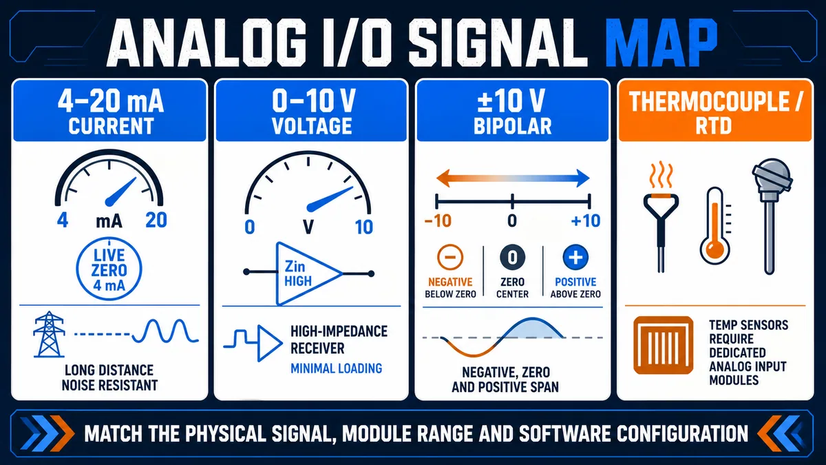
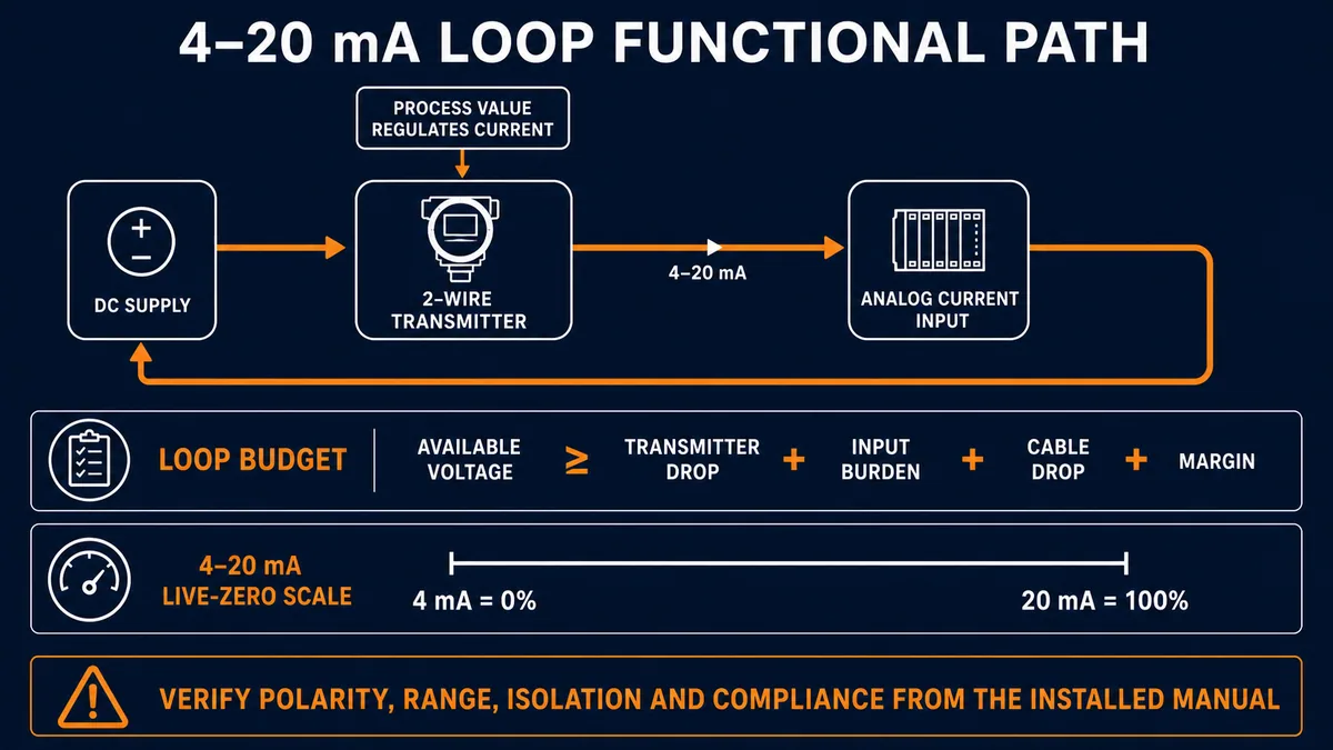
Four-to-twenty milliamp current loops provide a live zero: 4 mA represents the lower measurement endpoint while current near zero can indicate lost loop power or an open circuit. NI notes that the series current is common around a single loop and that current signaling is useful over long industrial cable runs. Voltage inputs use a potential difference and a high-impedance receiver; lead resistance, reference potential, common-mode limits and induced noise therefore require different attention. Bipolar ranges represent values below and above an engineering zero.

Thermocouples and RTDs are sensor technologies, not generic voltage inputs. Thermocouples require the correct type, polarity, extension wiring and cold-junction treatment. RTDs require the correct element type, connection arrangement and lead compensation. Use modules and configuration intended for the exact sensor.

Signal family	Typical representation	Design strength	Boundary to verify
4–20 mA	live-zero unipolar process span	long-run current signaling and low-end fault discrimination	loop power, burden, polarity, isolation and diagnostics
0–20 mA	zero-current lower endpoint	simple unipolar current span	zero process cannot be separated from an open loop by value alone
0–10 V	unipolar voltage span	common for local devices and commands	reference/common, input impedance, drop, common mode and noise
±10 V	bipolar value around zero	direction or signed command/measurement	sign, common mode and negative-range support
thermocouple	small sensor voltage by type	wide temperature measurement families	type, polarity, cold junction, compensation wire and module support
RTD	resistance related to temperature	stable temperature measurement	element curve, two/three/four-wire method and excitation

Distinguish active, passive and isolated interfaces

“Current input” does not reveal who supplies loop power. A two-wire transmitter is commonly loop-powered and regulates series current. A three- or four-wire transmitter may have separate power and source its output. An input can be passive, provide transmitter power, share a common across channels or be individually isolated. Those details control whether a proposed connection is valid and whether one channel can create a ground path for another.

Build the channel record from the actual manuals and drawings: source type, receiver type, supply, isolation boundary, reference/common, range, burden or input impedance, permitted common-mode voltage, shield termination philosophy and diagnostic capabilities.

Understand the 4–20 mA loop as a voltage budget

Current remains valid only while every device has enough voltage

The transmitter regulates current, but it needs operating voltage. The supply must cover the transmitter's minimum voltage, the analog input burden, cable drop, barriers or isolators, indicators and a design margin at the highest intended loop current and worst credible conditions. NI describes this as selecting a supply equal to or greater than the combined voltage drops. Too little available voltage can make the loop saturate or read low at the upper range.

For a conceptual 24 V loop, suppose the transmitter requires 12 V, the input drops 5 V at 20 mA, barriers and cable account for 3 V, and the design reserves 2 V. The required total is 22 V, leaving 2 V nominal margin. This is not a universal sizing example: minimum/maximum supply, temperature, fault limits, certification and exact burdens come from the installed product data.

Loop-budget term	What to obtain	Why it changes
supply at field condition	specified minimum at load, not label nominal only	regulation, loading, distribution and temperature
transmitter requirement	minimum operating voltage over intended current/environment	product electronics and optional display/features
analog input burden	product input resistance or voltage drop	range and channel design
barrier/isolator drop	exact channel and certification data	protective/interface design and load
cable/connection drop	loop resistance at condition and current	length, conductor, temperature and connections
design margin	engineered allowance	variation, uncertainty and maintainability

Live zero helps diagnosis but does not identify every cause

A 4 mA reading can be a healthy lower-range process value. A very low current can represent open wiring, lost transmitter power, reversed polarity, a failed transmitter, a tripped barrier or a test configuration. A current above the measurement span can represent a valid device alarm signal, real overrange, wrong range or an injected test. Use module diagnostics and transmitter status, not a single universal threshold. Schneider's TM3 diagnostics, Siemens S7-1200 G2 and Rockwell PointMax documentation use product- and configuration-specific limits.

Scale raw and electrical values into engineering units

Use a two-point linear map with explicit endpoints

For a linear signal, define the input lower endpoint Xlow, input upper endpoint Xhigh, engineering lower endpoint Ylow and engineering upper endpoint Yhigh:

Y = Ylow + (X − Xlow) × (Yhigh − Ylow) ÷ (Xhigh − Xlow)

For 4–20 mA representing 0–250 psi, Xlow = 4, Xhigh = 20, Ylow = 0 and Yhigh = 250. At 12 mA:

Y = 0 + (12 − 4) × 250 ÷ 16 = 125 psi

NI gives the equivalent straight-line method for a 0–200 psi example and derives its slope and intercept from the endpoints. The endpoint form above is often easier to review because the intended spans remain visible.

Injected/observed current	Fraction of 4–20 mA span	Ideal value for 0–250 psi	Review purpose
4 mA	0	0 psi	lower endpoint and live-zero offset
8 mA	0.25	62.5 psi	quarter-span linearity and data type
12 mA	0.50	125 psi	midpoint
16 mA	0.75	187.5 psi	upper-half slope
20 mA	1.00	250 psi	upper endpoint

Use the module's real data format, not an assumed raw range

Some modules return engineering current, normalized integers, percentages, floating-point values or vendor-specific counts. Others reserve ranges outside nominal span for overrange or diagnostics. Schneider documents product-dependent conversion of module data; Rockwell and Siemens manuals publish their own raw representations and status structures. Never assume that every 16-bit field means 0–65,535 usable counts or that 4 mA maps to zero.

If the installed module maps 4–20 mA to a documented raw span of RawLow through RawHigh, substitute those endpoints in the same formula. Preserve a wide enough intermediate data type to avoid integer truncation or overflow. Test below, at and above each endpoint. Version the range and transmitter engineering span together so a transmitter rerange does not silently leave the PLC scale wrong.

Scaling defect	Visible symptom	Discriminating check
0–20 assumption applied to 4–20 signal	lower endpoint shows 20% instead of 0%	compare configured electrical range and formula endpoints
wrong engineering upper range	correct zero, proportional span error	compare transmitter range record with PLC constants
integer division too early	stair-step or mostly zero result	inspect operation order and intermediate types
signed/unsigned mismatch	negative or large wraparound values	compare module data type and tag type
clamping before quality evaluation	failed loop appears as a valid endpoint	inspect raw/status path before limiter
duplicate scaling	HMI value wrong by stable factor	trace module, PLC and HMI conversion ownership

Evaluate resolution, accuracy, update time and filtering separately

More bits do not guarantee a more accurate measurement

Resolution describes the digital code width; accuracy describes closeness to the true value under specified conditions. NI explicitly distinguishes resolution, sensitivity, precision and accuracy and notes that noise and front-end circuitry can dominate nominal code width. A 16-bit module is not automatically more accurate than a 12-bit module. Range, gain/offset error, temperature drift, calibration interval, source impedance, common mode, input filter and system wiring all contribute.

The ideal code width is input span ÷ 2^bits only when all converter codes are used across that span. The real module may use fewer codes or encode diagnostic bands. Even an ideal small code width is not the system uncertainty. Build an error budget from the transmitter, signal conditioner, barriers, module, reference and environmental specifications when the application needs a quantified result.

Property	Meaning	It does not prove
resolution/bits	nominal discrete conversion levels	absolute accuracy or noise-free counts
accuracy	bounded deviation under stated conditions	repeatability outside those conditions
precision/repeatability	stability across repeated observations	closeness to the true process value
update time	how often channel data is refreshed	useful bandwidth after filtering/multiplexing
input filter	attenuation of specified signal content	removal of every interference mechanism
isolation/common mode	permitted separation/reference behavior	unlimited voltage or immunity to all ground faults

Filter only after fixing connection and quality faults

A low-pass filter or average can reduce high-frequency variation, but it trades bandwidth and adds delay. NI's field-wiring guidance notes that filtering is not a substitute for correct interconnection. Choose bandwidth from process dynamics and protection/control needs. Store both raw and filtered trends during commissioning so a filter does not hide dropouts, steps or aliasing. Alarms that require prompt response may need raw quality and a separately conditioned process value.

Treat channel diagnostics as data, not decoration

Pair every value with quality and range status

Schneider TM3 modules expose channel status codes for normal, configuration, external power, high/low wiring, hardware and extended-zone conditions. Rockwell PointMax exposes tags such as overrange and underrange and documents configurable behavior during open wire. Siemens S7-1200 G2 publishes product-specific open-wire behavior for 4–20 mA ranges. Thresholds differ, so the PLC should use the exact module's status semantics.

Represent an analog point as a small record: raw/electrical value, engineering value, quality, under/overrange, wire-break or channel fault, timestamp, source and simulation/force state. HMI presentation should show bad or uncertain quality visibly rather than displaying a normal-looking last value without indication.

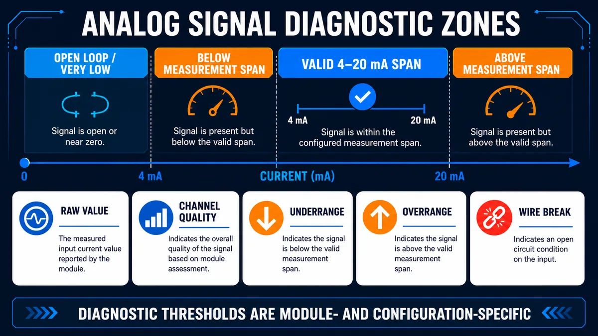
Raw/status pattern	Competing explanations	Next evidence
near zero current	open loop, lost supply, reversed circuit, failed device or test state	transmitter power/status and approved loop-segment check
below 4 mA but not open	device alarm/underrange, real below-scale process, calibration or range mismatch	transmitter indication/manual and channel diagnostic threshold
exactly at one endpoint for long periods	real saturated process, clamp, substituted value or frozen data	raw value, quality, timestamp and physical reference
above 20 mA	transmitter alarm/overrange, wrong range or injected signal	device status, calibrator record and configured module range
plausible but noisy	process variation, grounding/coupling, unstable supply or sensor	compare field display, loop current, module raw and neighboring channels
all channels shift together	shared common/supply/reference, module temperature or configuration	shared dependencies and independent reference measurement

Define bad-quality process behavior explicitly

When quality becomes bad, decide separately what the display, control strategy, alarms, historian and downstream consumers do. Options may include hold last with visible bad quality, substitute a defined value, suspend automatic control, transfer mode, or trip through a separately designed protective function. None is universally correct. A last good value can become dangerously stale; zero can be interpreted as a real low process; forcing maximum can create an opposite hazard.

Diagnose noise, offsets and unstable readings systematically

Start with topology and shared references

Compare one channel with neighboring channels, transmitter local indication, an independent calibrated reference and the process timeline. A single-channel issue points toward its transmitter, circuit, configuration or module channel. Multiple aligned shifts suggest a shared supply, common, grounding, reference, environmental or module cause. A value that changes with motor or drive switching suggests coupling or shared-reference behavior, but timing alone is not proof.

Use the installed manufacturer guidance for cable type, separation, shield treatment, commoning and grounding. Siemens guidance recommends separating low-voltage signal cables from high-energy conductors and using shielded wiring for noise protection, but exact shield termination depends on the system and EMC design. Do not casually add a second ground connection; it can create a ground loop or violate isolation/common-mode limits.

Noise/offset signature	High-value comparison	Possible class
periodic 50/60 Hz ripple	spectral/timed trend, reference and grounding topology	power-frequency coupling or ground loop
step when VFD/contactor switches	raw value and shared routing/reference at event	electromagnetic coupling or supply/common disturbance
stable offset across full span	independent calibrator at endpoints	scaling offset, transmitter zero, module offset or reference
increasing error near high current	loop voltage and budget at 20 mA	insufficient compliance/headroom or resistance
noisy only when multiple channels active	multiplex settling/source impedance or shared common	module/channel interaction and source characteristics
slow response without raw noise	configured filter/update and transmitter damping	intentional bandwidth reduction, not wiring noise

Avoid filtering a broken signal into plausibility

Filtering can turn intermittent open circuits into smooth but false trends. Evaluate channel quality and extreme raw excursions before the filter. Count dropouts and track maximum slew so maintenance can see a deteriorating connection even if the operator display remains stable. Apply debounce to diagnostic declaration only when the module behavior, process risk and timing justify it.

PLC analog output example: 4–20 mA valve or VFD

Define the complete command contract before writing a raw value

An analog output begins with an engineering setpoint. Apply process limits, rate limits, mode ownership and bumpless-transfer behavior before converting to module command data. Confirm the module configuration produces the intended voltage/current range. Then verify the receiver—such as a valve positioner or drive—interprets the same range and action direction. Finally, use independent process feedback where the consequence requires proof.

At 50% of a 4–20 mA output span, the ideal electrical command is 12 mA. That does not prove the valve is half open or the process is at half capacity. Positioner calibration, actuator mechanics, installed characteristic, stiction, downstream conditions and process nonlinearity remain separate.

Use this vendor-neutral worked case:

• The application owns a 0…100% valve-demand variable.
• The authorized module documentation says the configured 4…20 mA range maps its lower electrical endpoint to raw 0 and upper endpoint to raw 27648.
• Manual, automatic, maintenance and fault modes have one explicit command owner.
• Normal operation clamps demand to the engineered limits and applies a reviewed slew-rate limit before conversion.
• The valve positioner is configured for the same 4…20 mA direct-acting range.
• Independent position or process feedback proves response; the output command is not treated as proof of movement.

The general output equation is:

Fraction = (Command − EngineeringLow) ÷ (EngineeringHigh − EngineeringLow)

RawOutput = RawLow + Fraction × (RawHigh − RawLow)

ElectricalOutput = SignalLow + Fraction × (SignalHigh − SignalLow)

At a 62.5% command in this example:

Fraction = (62.5 − 0) ÷ (100 − 0) = 0.625

RawOutput = 0 + 0.625 × 27648 = 17280

Current = 4 mA + 0.625 × 16 mA = 14 mA

Engineering command	Fraction	Illustrative raw 0…27648	Ideal 4–20 mA	Ideal 0–10 V
0%	0.00	0	4 mA	0 V
25%	0.25	6912	8 mA	2.5 V
50%	0.50	13824	12 mA	5 V
62.5%	0.625	17280	14 mA	6.25 V
75%	0.75	20736	16 mA	7.5 V
100%	1.00	27648	20 mA	10 V

The two electrical columns are alternative configured examples, not simultaneous outputs. A current channel and a voltage channel have different terminals, load/compliance limits, reference behavior and fault signatures. Never change signal type by editing only the formula.

Use a bounded program pattern rather than a magic multiplier

The following Structured Text is illustrative IEC-style pseudocode. Adapt function signatures, numeric types, rounding and output tags to the approved platform. RawLow and RawHigh must come from the exact module's configured data representation.

(* Vendor-neutral analog-output scaling pattern. *)
IF OutputPermitted AND ModuleHealthy THEN
    CommandBounded := LIMIT(EngineeringLow, CommandRequested, EngineeringHigh);
    CommandRamped := ApplyApprovedRateLimit(
        Target := CommandBounded,
        Previous := CommandRamped,
        RisePerCycle := RiseLimit,
        FallPerCycle := FallLimit
    );

    SpanValid := EngineeringHigh > EngineeringLow;
    IF SpanValid THEN
        Fraction := (CommandRamped - EngineeringLow)
                    / (EngineeringHigh - EngineeringLow);
        RawReal := RawLow + Fraction * (RawHigh - RawLow);
        AnalogOutputRaw := REAL_TO_DINT(RawReal);
    ELSE
        ScalingFault := TRUE;
        AnalogOutputRaw := DefinedFaultRaw;
    END_IF;
ELSE
    AnalogOutputRaw := DefinedNotPermittedRaw;
END_IF;

The pattern deliberately keeps permission, module health, limits, slew, span validation and numeric conversion visible. A production implementation also needs documented manual/automatic transfer, startup initialization, controller stop behavior, module fault reaction, communication loss, receiver fault, force/simulation tracking and restoration. A single Command × 276.48 expression hides those decisions and can overflow, truncate or continue commanding an unsafe state.

Translate the example into ladder logic without losing the contract

In ladder, implement the same sequence as explicit rungs or reusable blocks: select the authorized command owner; evaluate permissives; clamp engineering demand; apply the approved rate limiter; normalize/scaling with wide intermediate types; convert once at the output boundary; then move the result to the mapped analog-output tag. Put diagnostics and fallback selection beside that path, not in an unrelated routine.

Do not place an unqualified HMI number directly into the output word. The HMI is a request source. The PLC application decides whether that source owns the command, whether the value is in range, whether the process permits the change and what should happen if communication becomes stale.

Program layer	Required decision	Evidence during review
source ownership	auto, manual, maintenance or fallback—exactly one writer	command-source state and cross-reference
process permission	which interlocks and modes allow an analog command	cause-and-effect or control narrative
engineering bounds	minimum, maximum and action direction	equipment/process specification
rate behavior	rise/fall limits and scan/task basis	trend of requested versus ramped command
scaling	electrical and raw endpoints, types and rounding	endpoint calculation plus module manual
output mapping	exact channel/tag and configured range	project hardware configuration and I/O map
feedback	receiver indication, position or process response	independent measurement with timestamps
failure reaction	program, module, network and power states	controlled negative/recovery test results

Prove the VFD or valve response at six boundaries

For a VFD, confirm its active reference source, analog-input mode, low/high electrical points, minimum/maximum speed, start/stop ownership and signal-loss reaction. A correct 14 mA command can still produce zero speed if the drive is in keypad mode, waiting for a run permissive, clamped by a minimum-frequency rule or faulted. For a valve, confirm the positioner's signal range, action direction, calibration, air/energy supply, mechanical travel and any split-range or characterization.

Test the engineering request, scaled raw command, module/channel status, measured signal, receiver display, actuator response and process feedback together. At minimum use lower endpoint, midpoint, upper endpoint, one off-midpoint such as 62.5%, a denied-command state and the specified loss/recovery case. Record tolerances and settling time; do not expect a calibrated field loop to equal the mathematical ideal to infinite precision.

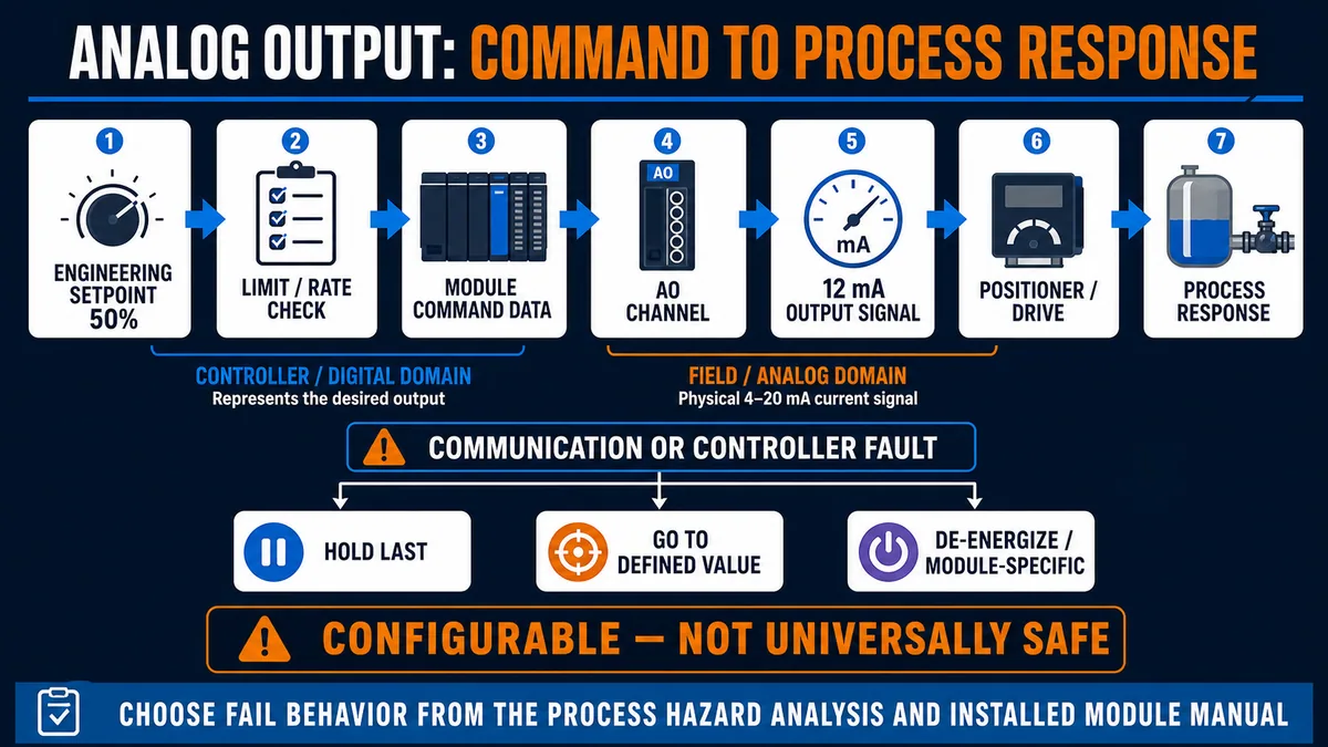
Output state	Design questions	Verification evidence
manual-to-auto transfer	who owns command and is transfer bumpless?	pre/post command, mode and process trend
configured minimum/maximum	do electrical and engineering limits agree?	endpoint command, measured output and receiver indication
controller/program mode	hold, defined value or module-specific reaction?	exact configuration and controlled recovery test
network/connection fault	when does module detect loss and what value follows?	fault timing, module status and physical output
module/channel fault	can output freeze, drop or report uncertainty?	module diagnostics and independent signal/process evidence
power loss/recovery	what does receiver and actuator physically do?	energy-source, actuator and process response test

Choose fail behavior from process hazards, not habit

Rockwell manuals document configurable output reactions such as hold-last or a defined fault value for particular modules. Those are capabilities, not universal safety recommendations. A cooling valve may need one response while a fuel valve requires another. The actuator's mechanical fail action, process inventory, energy source and independent protection all matter. Specify, review and test controller fault, network fault, module fault and power-loss behavior independently.

Distinguish PWM from a true analog output

A pulse train is not automatically a voltage or current signal

Some PLCs advertise pulse-width modulation (PWM) on a digital or high-speed output. PWM encodes a duty ratio in switching time. A true analog output produces a specified continuous voltage or current through a defined converter and output stage. A receiving device designed for PWM may interpret duty directly; an analog receiver may require an engineered filter/interface, and ripple, frequency, loading, isolation and fault behavior then become part of the design.

Do not connect a PWM output to a 0–10 V or 4–20 mA input merely because an average meter appears to show a proportional value. Verify the PLC output electrical type, switching frequency, receiver input model and any approved signal converter. When the task is stable instrumentation or actuator command, a supported analog module is usually the clearer diagnostic boundary.

Feature	PWM digital output	True analog output
encoded quantity	duty cycle and frequency	continuous current or voltage level
receiver requirement	PWM-compatible input or engineered conversion	matching current/voltage input range
likely diagnostics	digital output and pulse configuration	channel status, range, open load/product-specific faults
main quality concerns	frequency, jitter, ripple and filter response	accuracy, resolution, burden, common mode and noise
failure interpretation	stuck high/low or missing pulses	hold, defined value, open circuit or module-specific state

Commission analog I/O with an endpoint and quality matrix

Verify identity and configuration before applying signals

Record module/catalog, hardware and firmware revision, channel number, physical signal, source/receiver type, isolation group, configured range, data format, engineering range, diagnostic enablement, filter/update, fail behavior, PLC tag and HMI/historian consumer. Confirm that drawings and transmitter calibration records match the configuration.

Under an approved test plan, verify lower endpoint, midpoint, upper endpoint and diagnostic behavior. Test the transmitter-to-PLC chain and the module channel separately only when the isolation method is controlled. For outputs, compare requested engineering value, module data, measured signal, receiver indication and process result. Remove simulations/forces and prove restoration explicitly.

Commissioning case	Applied/observed condition	Required evidence	Acceptance focus
lower endpoint	documented lower signal	raw, quality and engineering lower value	correct offset and live-zero interpretation
midpoint	50% signal	proportional raw and engineering midpoint	slope and data type
upper endpoint	documented upper signal	raw, quality and engineering upper value	span and headroom
below/above span	approved simulator/test function	exact module status plus unclamped raw	product-specific diagnostic handling
open-loop test	only if approved and safe	wire-break/open status and consumer reaction	bad quality is visible, not a plausible zero
noisy/step response	controlled source transition	raw and filtered trend with timing	filter/update match process requirement
analog output endpoints	bounded authorized commands	module command, physical signal and receiver response	action, range and direction
communication recovery	controlled loss/restore	configured fail value and restart transfer	no unexpected bump or stale command
force/simulation removal	normal source restored	force inventory clear and live timestamp/quality	no hidden test state remains

Use three-point checks and independent references

One test point cannot separate offset from span error. Three points reveal endpoint, slope and nonlinearity clues. Use calibrated equipment appropriate to the required uncertainty and document its identity, range and due date. Compare against the complete system tolerance rather than demanding the PLC display match the calibrator's last digit.

Troubleshoot from field quantity to process result

Find the first boundary where evidence diverges

For an input, compare the physical process/reference, transmitter local value, loop signal, module raw/status, scaled value, filtered value, HMI/historian display and control action. For an output, reverse the chain from requested setpoint through module command, physical current/voltage, receiver indication, actuator position and process response. The earliest credible mismatch localizes the next test boundary.

Symptom	First comparison	Likely boundary classes
raw value bad and transmitter display good	loop signal/status versus transmitter output	loop power, wiring, barrier, input configuration or channel
raw value good, engineering value wrong	raw endpoints versus scaling constants/types	PLC scaling or range ownership
PLC value good, HMI value wrong	published tag versus HMI scaling/units/quality	display mapping or duplicate conversion
only filtered value lags	raw versus filter/update settings	intended or excessive conditioning
output command changes, measured signal does not	module data/status versus physical output	channel configuration, power, load or module fault
signal changes, actuator does not	measured signal versus receiver/actuator state	receiver range, mode, mechanics or energy source
actuator moves, process does not respond	position versus independent process evidence	process path, coupling, valve/pump/load or sensor

Preserve timestamps, quality and change history

Analog faults are often intermittent. Trend raw and engineering values, quality/status, supply or common dependencies, mode, output command and relevant equipment events with aligned timestamps. Record module or transmitter replacement, calibration, range edits, shield/ground changes, cabinet work and nearby drive or motor changes. A stable offset after a range edit is different from bursts synchronized to switching.

For more general digital and field-I/O boundaries, use PLC input and output troubleshooting. This page remains the canonical owner for analog ranges, scaling, measurement quality and current/voltage diagnostics.

Diagnostic answer map for PLC analog I/O

Question a technician or AI assistant may ask	Short, extractable answer	Evidence that decides it
How do I scale 4–20 mA to engineering units?	Map 4 mA to the engineering lower endpoint and 20 mA to the upper endpoint using a two-point linear formula, then test at least three points.	configured electrical/raw endpoints and transmitter range record
What should 12 mA equal on a 0–250 psi transmitter?	Ideally 125 psi because 12 mA is 50% of the 4–20 mA span.	transmitter is actually ranged 0–250 psi and channel is configured 4–20 mA
Why does a 4–20 mA input read zero?	Candidates include an open loop, lost power, reversed polarity, failed device, wrong configuration or test state; zero is not a valid normal endpoint for a live-zero range.	channel quality, transmitter power/status and approved loop evidence
Is 16-bit analog input more accurate than 12-bit?	Not necessarily; resolution is code width, while accuracy also depends on converter/front-end error, noise, calibration, range and system components.	exact specifications and system uncertainty budget
Why is the analog value noisy when a motor runs?	Coupling, shared supply/common, grounding, routing or real process vibration are candidates; align raw trends with switching and compare independent references.	topology, timestamps, neighboring channels and field reference
Should bad analog quality be clamped to zero?	Not automatically; zero may look like a valid low process. Preserve bad quality and choose consumer behavior from process risk.	module status, control consequence and hazard analysis
Is PWM the same as analog output?	No. PWM is a switched duty-cycle signal; a true analog output produces a specified continuous current or voltage.	PLC output electrical specification and receiver requirements
What should an analog output do on communication loss?	Hold, move to a defined value or another module-specific reaction may be configurable; the least hazardous choice is process-specific.	hazard analysis, actuator behavior and installed module manual

Frequently asked questions

What is a PLC analog output example?

A PLC can send a 0…100% speed or valve command through a configured 4…20 mA output. If the exact module maps that electrical span to raw 0…27648, a 62.5% request becomes raw 17280 and ideally measures 14 mA. The program must also qualify ownership, limits, slew, module status, receiver configuration, failure behavior and independent process response.

Why is 4–20 mA common in industrial control?

It provides a live zero at 4 mA, supports two-wire loop-powered transmitters, carries the same series current through the loop and is practical over long industrial cable runs. Its value still depends on adequate loop voltage, compatible source/receiver types, isolation/common-mode limits and correct diagnostics.

How do you convert 4–20 mA to a percentage?

Use (mA − 4) ÷ 16 × 100. Thus 4 mA is 0%, 12 mA is 50% and 20 mA is 100% for the nominal span. Evaluate channel status before treating a below- or above-span result as a valid percentage.

What is the difference between 0–10 V and 4–20 mA PLC inputs?

A voltage input measures potential relative to its configured reference and commonly has high input impedance. A current input measures series loop current and imposes a defined burden. They have different source, common-mode, drop, noise, open-circuit and wiring requirements and cannot be swapped through software scaling.

What does analog-input resolution mean?

Resolution is the smallest ideal digital code step over a configured converter span. It does not equal absolute accuracy. Noise, offset/gain error, temperature, calibration, filtering, source and module front end can make the useful measurement uncertainty much larger than one ideal count.

Why does a 4–20 mA signal show less than 4 mA?

The process may be below the calibrated span, the transmitter may intentionally signal a diagnostic state, or the loop may have a power, polarity, wiring, burden, range or device fault. Interpret the value with the exact transmitter and module diagnostic rules; do not apply a universal fault threshold.

Should PLC analog scaling clamp values to 0–100 percent?

Clamping can protect downstream arithmetic, but retain the unclamped value and quality for diagnostics. If clamping happens before status evaluation, an open or overrange circuit can masquerade as a healthy endpoint. Define display, control and alarm behavior separately.

How do you troubleshoot an unstable PLC analog input?

Compare raw value, status, transmitter indication, independent reference, neighboring channels, shared supply/common and switching events. Verify topology, range, isolation, routing and shield/ground design from the manuals. Apply filtering only after connection and quality causes are evaluated.

Can a PLC PWM output replace a 0–10 V analog output?

Only when the receiving device explicitly accepts PWM or an engineered interface converts the pulses with acceptable ripple, response, loading, isolation and fault behavior. An average multimeter reading does not establish compatibility. A supported analog module gives a defined continuous output and clearer diagnostics.

What happens to a PLC analog output when communications fail?

It depends on module and configuration. Some modules can hold the last value or move to a defined fault value; power loss and channel faults may behave differently. Select and test each response using the process hazard analysis, receiver/actuator behavior and exact installed manual.

Sources, review scope, and limitations

This guide synthesizes functional and diagnostic principles from the primary sources below. Product examples demonstrate why range, data and diagnostic behavior must be version-specific; they are not interchangeable settings or universal thresholds. The conceptual images omit terminal-level wiring and do not replace engineered drawings.

1. Siemens S7-1200 G2 System Manual (2025) — current analog signal-board ranges, data representation, two-wire transmitter examples and open-wire behavior.
2. Siemens S7-1500 Analog Value Processing Function Manual — analog representation, wire-break configuration and processing concepts.
3. Siemens S7-1200 Functional Safety Manual: wiring and grounding guidance — cable separation, shielding, grounding and isolation boundaries; cited for general installation context, not standard I/O as a safety function.
4. Rockwell Automation PointMax Analog I/O Modules User Manual — channel configuration, overrange/underrange tags, open-wire choices and current-input diagnostics.
5. Rockwell Automation FLEX I/O Isolated Analog Modules User Manual — isolated input/output formats, ranges and product-specific underrange behavior.
6. Rockwell Automation FLEX I/O Analog Modules User Manual — range selection, module data and configurable analog-output safe-state values.
7. Rockwell Automation ControlLogix High-Resolution Analog I/O User Manual — current analog module tags, channel status and configurable program/fault reactions.
8. Schneider Electric TM3TI4/TM3TI4G configuration — supported current, voltage, thermocouple and RTD ranges plus physical/configuration compatibility warning.
9. Schneider Electric TM3 Analog I/O Diagnostics — channel-status codes and product/range-specific diagnostic zones.
10. Schneider Electric TM3 General Description — current module range, resolution and channel-type examples.
11. NI 4–20 mA Current Loop Fundamentals — current-loop components, live zero, loop voltage budget, shunt burden and isolation context.
12. NI: How Can I Scale My 4–20 mA Sensor Data? — two-point linear scaling example and endpoint method.
13. NI Analog Sample Quality: Accuracy, Sensitivity, Precision and Noise — measurement terminology, accuracy contributors and noise reduction limits.
14. NI Field Wiring and Noise Considerations for Analog Signals — connection topology, common mode, noise, averaging and bandwidth tradeoffs.
15. OSHA 29 CFR 1910.147, Control of Hazardous Energy — energy-isolation definitions and hazardous-energy control requirements.